当前位置:网站首页>3、 Gradient descent solution θ
3、 Gradient descent solution θ
2022-04-23 14:40:00 【Beyond proverb】
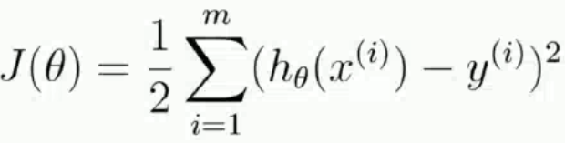
One 、 Get the objective function J(θ), The solution makes J(θ) The youngest θ value
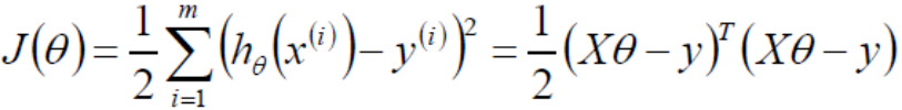
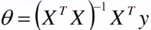
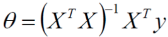
Find the minimum value of the objective function by the least square method
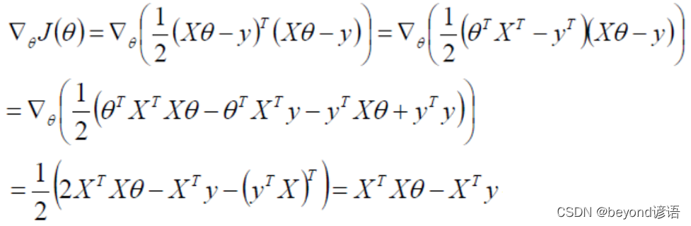
Let the partial guide be 0 You can solve the minimum θ value , namely 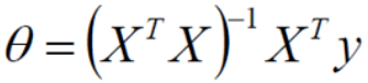
Two 、 Determine as convex function
Convex functions need judgment methods , such as : Definition 、 First order conditions 、 Second order condition, etc . Using positive definiteness, the second-order condition is used .
A positive semidefinite must be a convex function , Opening up , Positive semidefinite must have a minimum
When judging with second-order conditions , Need to get Hessian matrix , according to Hessian The positive definiteness of determines the concavity and convexity of the function . such as Hessian Matrix positive semidefinite , The function is convex ;Hessian The matrix is positive definite , Strictly convex function
Hessian matrix : Hesse matrix (Hessian Matrix), Also known as Hessian matrix 、 Heather matrix 、 Hesse matrix, etc , It is a square matrix composed of the second partial derivatives of a function of several variables , Describes the local curvature of a function .
3、 ... and 、Hessian matrix
The Hesse matrix is determined by the objective function at point x A symmetric matrix consisting of the second partial derivatives at
Positive definite : Yes A The eigenvalues of are all positive numbers , that A It must be positive definite
improper : Non positive definite or semi positive definite
if A The eigenvalues of the ≥0, Then semidefinite , otherwise ,A Is non positive definite .
Yes J(θ) Find the second derivative of the loss function , What you get must be positive semidefinite , Because I do dot multiplication with myself .
Four 、 Analytic solution
The numerical solution is a numerical value calculated by some approximation under certain conditions , It can satisfy the equation under the given accuracy conditions , The analytical solution is the analytical formula of the equation ( Such as root formula and so on ), Is the exact solution of the equation , It can satisfy the equation with arbitrary accuracy .
5、 ... and 、 Gradient descent method
This course is similar to other courses , I won't go into details here . Gradient descent method
Gradient descent method : It is a method to find the optimal solution at the fastest speed .
technological process :
1, initialization θ, there θ It's a set of parameters , Initialization is random Then you can.
2, Solving gradient gradient
3,θ(t+1) = θ(t) - grand*learning_rate
there learning_rate Commonly used α It means the learning rate , It's a super parameter , Too big , If the step is too big, it is easy to shake back and forth ; Too small , A lot of iterations , Time consuming .
4,grad < threshold when , Iteration stop , convergence , among threshold It's also a super parameter
Hyperparameters : The parameters passed in by the user are required , If not, use the default parameters .
6、 ... and 、 Code implementation
Guide pack
import numpy as np
import matplotlib.pyplot as plt
Initialize sample data
#  It's quite random X dimension X1,rand Is a random uniform distribution
X = 2 * np.random.rand(100, 1)
#  Artificial settings, real Y A column of ,np.random.randn(100, 1) It's settings error,randn It's the standard Zhengtai distribution
y = 4 + 3 * X + np.random.randn(100, 1)
#  Integrate X0 and X1
X_b = np.c_[np.ones((100, 1)), X]
print(X_b)
""" [[1. 1.01134124] [1. 0.98400529] [1. 1.69201204] [1. 0.70020158] [1. 0.1160646 ] [1. 0.42502983] [1. 1.90699898] [1. 0.54715372] [1. 0.73002827] [1. 1.29651341] [1. 1.62559406] [1. 1.61745598] [1. 1.86701453] [1. 1.20449051] [1. 1.97722538] [1. 0.5063885 ] [1. 1.61769812] [1. 0.63034575] [1. 1.98271789] [1. 1.17275471] [1. 0.14718811] [1. 0.94934555] [1. 0.69871645] [1. 1.22897542] [1. 0.59516153] [1. 1.19071408] [1. 1.18316576] [1. 0.03684612] [1. 0.3147711 ] [1. 1.07570897] [1. 1.27796797] [1. 1.43159157] [1. 0.71388871] [1. 0.81642577] [1. 1.68275133] [1. 0.53735427] [1. 1.44912342] [1. 0.10624546] [1. 1.14697422] [1. 1.35930391] [1. 0.73655224] [1. 1.08512154] [1. 0.91499434] [1. 0.62176609] [1. 1.60077283] [1. 0.25995875] [1. 0.3119241 ] [1. 0.25099575] [1. 0.93227026] [1. 0.85510054] [1. 1.5681651 ] [1. 0.49828274] [1. 0.14520117] [1. 1.61801978] [1. 1.08275593] [1. 0.53545855] [1. 1.48276384] [1. 1.19092276] [1. 0.19209144] [1. 1.91535667] [1. 1.94012402] [1. 1.27952383] [1. 1.23557691] [1. 0.9941706 ] [1. 1.04642378] [1. 1.02114013] [1. 1.13222297] [1. 0.5126448 ] [1. 1.22900735] [1. 1.49631537] [1. 0.82234995] [1. 1.24810189] [1. 0.67549922] [1. 1.72536141] [1. 0.15290908] [1. 0.17069838] [1. 0.27173192] [1. 0.09084242] [1. 0.13085313] [1. 1.72356775] [1. 1.65718819] [1. 1.7877667 ] [1. 1.70736708] [1. 0.8037657 ] [1. 0.5386607 ] [1. 0.59842584] [1. 0.4433115 ] [1. 0.11305317] [1. 0.15295053] [1. 1.81369029] [1. 1.72434082] [1. 1.08908323] [1. 1.65763828] [1. 0.75378952] [1. 1.61262625] [1. 0.37017158] [1. 1.12323188] [1. 0.22165802] [1. 1.69647343] [1. 1.66041812]] """
#  Conventional equation solving theta
theta_best = np.linalg.inv(X_b.T.dot(X_b)).dot(X_b.T).dot(y)
print(theta_best)
""" [[3.9942692 ] [3.01839793]] """
#  Create... In the test set X1
X_new = np.array([[0], [2]])
X_new_b = np.c_[(np.ones((2, 1))), X_new]
print(X_new_b)
y_predict = X_new_b.dot(theta_best)
print(y_predict)
""" [[1. 0.] [1. 2.]] [[ 3.9942692 ] [10.03106506]] """
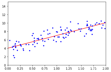
mapping
plt.plot(X_new, y_predict, 'r-')
plt.plot(X, y, 'b.')
plt.axis([0, 2, 0, 15])
plt.show()
7、 ... and 、 Complete code
import numpy as np
import matplotlib.pyplot as plt

#  It's quite random X dimension X1,rand Is a random uniform distribution
X = 2 * np.random.rand(100, 1)
#  Artificial settings, real Y A column of ,np.random.randn(100, 1) It's settings error,randn It's the standard Zhengtai distribution
y = 4 + 3 * X + np.random.randn(100, 1)

#  Integrate X0 and X1
X_b = np.c_[np.ones((100, 1)), X]
print(X_b)

#  Conventional equation solving theta
theta_best = np.linalg.inv(X_b.T.dot(X_b)).dot(X_b.T).dot(y)
print(theta_best)

#  Create... In the test set X1
X_new = np.array([[0], [2]])
X_new_b = np.c_[(np.ones((2, 1))), X_new]
print(X_new_b)
y_predict = X_new_b.dot(theta_best)
print(y_predict)

# mapping
plt.plot(X_new, y_predict, 'r-')
plt.plot(X, y, 'b.')
plt.axis([0, 2, 0, 15])
plt.show()
版权声明
本文为[Beyond proverb]所创,转载请带上原文链接,感谢
https://yzsam.com/2022/04/202204231436591095.html
边栏推荐
- 555定时器+74系列芯片搭建八路抢答器,30s倒计时,附Proteus仿真等
- 一个月把字节,腾讯,阿里都面了,写点面经总结……
- Branch statement of process control
- 成都控制板设计提供_算是详细了_单片机程序头文件的定义、编写及引用介绍
- Sed learning for application
- C语言知识点精细详解——数据类型和变量【2】——整型变量与常量【1】
- 51 MCU flowers, farmland automatic irrigation system development, proteus simulation, schematic diagram and C code
- 初始c语言大致框架适合复习和初步认识
- MDS55-16-ASEMI整流模块MDS55-16
- On the insecurity of using scanf in VS
猜你喜欢
PCIe X1 插槽的主要用途是什么?

Qt界面优化:Qt去边框与窗体圆角化
L'externalisation a duré quatre ans.

TLC5615 based multi-channel adjustable CNC DC regulated power supply, 51 single chip microcomputer, including proteus simulation and C code
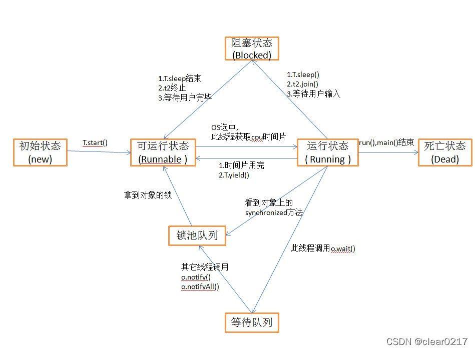
线程同步、生命周期
ASEMI三相整流桥和单相整流桥的详细对比
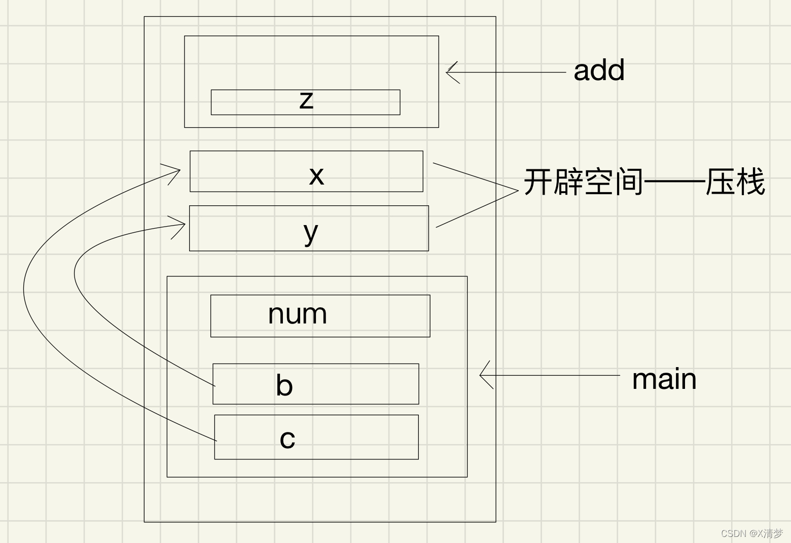
Parameter stack pressing problem of C language in structure parameter transmission
![[detailed explanation of factory mode] factory method mode](/img/56/04fa84d0b5f30e759854a39afacff2.png)
[detailed explanation of factory mode] factory method mode
Design of single chip microcomputer Proteus for temperature and humidity monitoring and alarm system of SHT11 sensor (with simulation + paper + program, etc.)
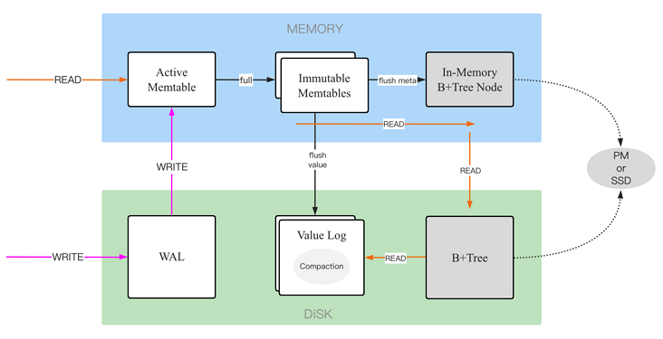
LotusDB 设计与实现—1 基本概念
随机推荐
c语言在结构体传参时参数压栈问题
L'externalisation a duré quatre ans.
流程控制之分支语句
一篇博客让你学会在vscode上编写markdown
拼接hql时,新增字段没有出现在构造方法中
select 同时接收普通数据 和 带外数据
Qt界面优化:鼠标双击特效
关于在vs中使用scanf不安全的问题
【Proteus仿真】自动量程(范围<10V)切换数字电压表
8.4 循环神经网络从零实现
Nacos uses demo as configuration center (IV)
线程同步、生命周期
如何打开Win10启动文件夹?
8.5 循环神经网络简洁实现
epoll 的EPOLLONESHOT 事件———实例程序
单相交交变频器的Matlab Simulink建模设计,附Matlab仿真、PPT和论文等资料
Design of single chip microcomputer Proteus for temperature and humidity monitoring and alarm system of SHT11 sensor (with simulation + paper + program, etc.)
OpenFaaS实战之四:模板操作(template)
Electronic perpetual calendar of DS1302_ 51 single chip microcomputer, month, day, week, hour, minute and second, lunar calendar and temperature, with alarm clock and complete set of data
MQ-2和DS18B20的火灾温度-烟雾报警系统设计,51单片机,附仿真、C代码、原理图和PCB等