当前位置:网站首页>目标检测——LeNet
目标检测——LeNet
2022-08-11 05:23:00 【壹万1w】
目标检测——LeNet
demo的流程
- model.py ——定义LeNet网络模型
- train.py ——加载数据集并训练,训练集计算loss,测试集计算accuracy,保存训练好的网络参数
- predict.py——得到训练好的网络参数后,用自己找的图像进行分类测试
目录
1. model.py
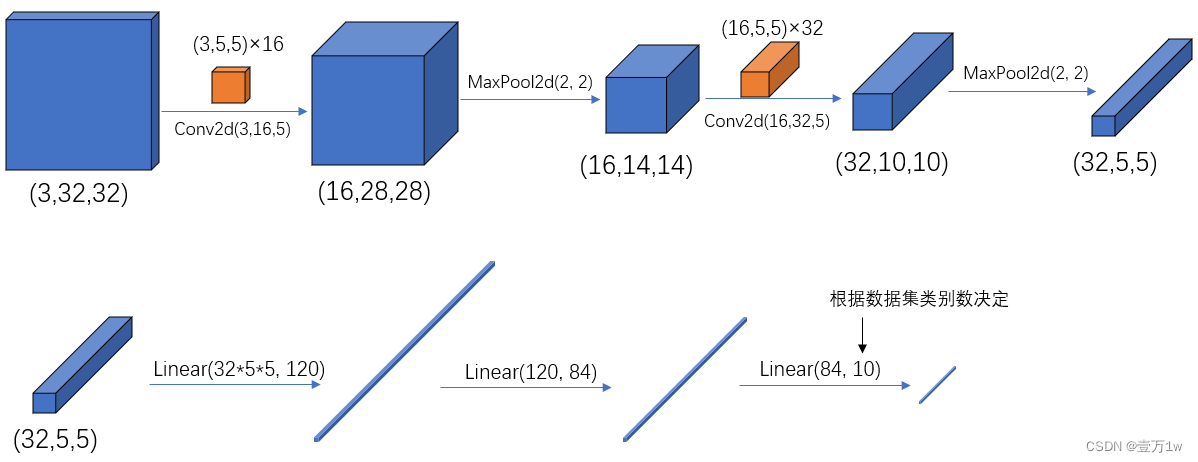
先给出代码,模型是基于LeNet做简单修改,层数很浅,容易理解:
# 使用torch.nn包来构建神经网络.
import torch.nn as nn
import torch.nn.functional as F

class LeNet(nn.Module): 					# 继承于nn.Module这个父类
    def __init__(self):						# 初始化网络结构
        super(LeNet, self).__init__()    	# 多继承需用到super函数
        self.conv1 = nn.Conv2d(3, 16, 5)
        self.pool1 = nn.MaxPool2d(2, 2)
        self.conv2 = nn.Conv2d(16, 32, 5)
        self.pool2 = nn.MaxPool2d(2, 2)
        self.fc1 = nn.Linear(32*5*5, 120)
        self.fc2 = nn.Linear(120, 84)
        self.fc3 = nn.Linear(84, 10)

    def forward(self, x):			 # 正向传播过程
        x = F.relu(self.conv1(x))    # input(3, 32, 32) output(16, 28, 28)
        x = self.pool1(x)            # output(16, 14, 14)
        x = F.relu(self.conv2(x))    # output(32, 10, 10)
        x = self.pool2(x)            # output(32, 5, 5)
        x = x.view(-1, 32*5*5)       # output(32*5*5)
        x = F.relu(self.fc1(x))      # output(120)
        x = F.relu(self.fc2(x))      # output(84)
        x = self.fc3(x)              # output(10)
        return x
需注意:
- pytorch 中 tensor(也就是输入输出层)的 通道排序为:
[batch, channel, height, width] - pytorch中的卷积、池化、输入输出层中参数的含义与位置,如下图:
1.1 卷积 Conv2d
我们常用的卷积(Conv2d)在pytorch中对应的函数是:
torch.nn.Conv2d(in_channels, out_channels, kernel_size, stride=1, padding=0, dilation=1, groups=1, bias=True, padding_mode='zeros')
一般使用时关注以下几个参数即可:
- in_channels:输入特征矩阵的深度。如输入一张RGB彩色图像,那in_channels=3
- out_channels:输入特征矩阵的深度。也等于卷积核的个数,使用n个卷积核输出的特征矩阵深度就是n
- kernel_size:卷积核的尺寸。可以是int类型,如3 代表卷积核的height=width=3,也可以是 tuple类型如(3, 5)代表卷积核的height=3,width=5
- stride:卷积核的步长。默认为1,和kernel_size一样输入可以是int型,也可以是tuple类型
- padding:补零操作,默认为0。可以为int型如1即补一圈0,如果输入为tuple型如(2, 1) 代表在上下补2行,左右补1列。
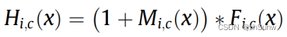
附上pytorch官网上的公式: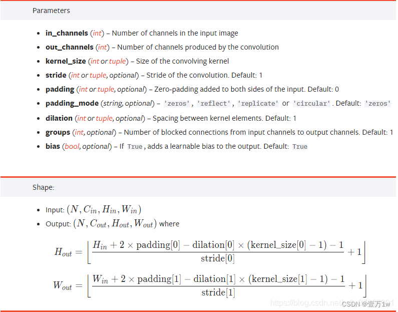
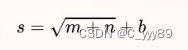
经卷积后的输出层尺寸计算公式为: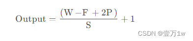
- 输入图片大小 W×W(一般情况下Width=Height)
- Filter大小 F×F
- 步长 S
- padding的像素数 P
若计算结果不为整数呢?pytorch中的卷积操作详解
1.2 池化 MaxPool2d
最大池化(MaxPool2d)在 pytorch 中对应的函数是:
MaxPool2d(kernel_size, stride)
1.3 Tensor的展平:view()
注意到,在经过第二个池化层后,数据还是一个三维的Tensor (32, 5, 5),需要先经过展平后(3255)再传到全连接层:
  x = self.pool2(x)            # output(32, 5, 5)
  x = x.view(-1, 32*5*5)       # output(32*5*5)
  x = F.relu(self.fc1(x))      # output(120)
1.4 全连接 Linear
全连接( Linear)在 pytorch 中对应的函数是:
Linear(in_features, out_features, bias=True)
2. train.py
2.1 导入数据集
导入包
import torch
import torchvision
import torch.nn as nn
from model import LeNet
import torch.optim as optim
import torchvision.transforms as transforms
import matplotlib.pyplot as plt
import numpy as np
import time
数据预处理
对输入的图像数据做预处理,即由shape (H x W x C) in the range [0, 255] → shape (C x H x W) in the range [0.0, 1.0]
transform = transforms.Compose(
    [transforms.ToTensor(),
     transforms.Normalize((0.5, 0.5, 0.5), (0.5, 0.5, 0.5))])
数据集介绍
利用torchvision.datasets函数可以在线导入pytorch中的数据集,包含一些常见的数据集如MNIST等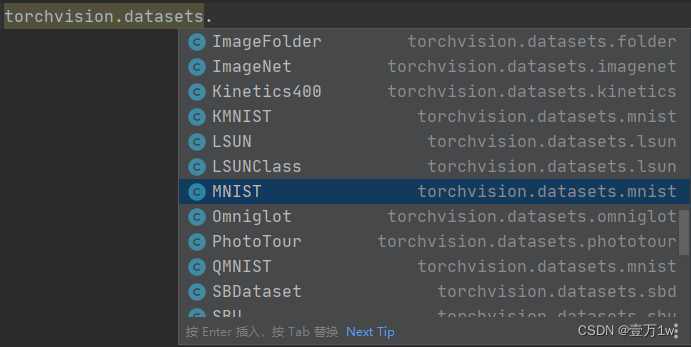
此demo用的是CIFAR10数据集,也是一个很经典的图像分类数据集,由 Hinton 的学生 Alex Krizhevsky 和 Ilya Sutskever 整理的一个用于识别普适物体的小型数据集,一共包含 10 个类别的 RGB 彩色图片。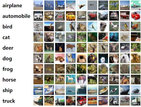
导入、加载 训练集
# 导入50000张训练图片
train_set = torchvision.datasets.CIFAR10(root='./data', 	 # 数据集存放目录
										 train=True,		 # 表示是数据集中的训练集
                                        download=True,  	 # 第一次运行时为True,下载数据集,下载完成后改为False
                                        transform=transform) # 预处理过程
# 加载训练集,实际过程需要分批次(batch)训练
train_loader = torch.utils.data.DataLoader(train_set, 	  # 导入的训练集
										   batch_size=50, # 每批训练的样本数
                                          shuffle=False,  # 是否打乱训练集
                                          num_workers=0)  # 使用线程数,在windows下设置为0
导入、加载 测试集
# 导入10000张测试图片
test_set = torchvision.datasets.CIFAR10(root='./data',  #放在根目录的data文件夹下
										train=False,	# 表示是数据集中的测试集
                                        download=False,transform=transform) #下载好后要把download改成false
# 加载测试集,并且分批次训练
test_loader = torch.utils.data.DataLoader(test_set,
										  batch_size=10000, # 每批用于验证的样本数
										  shuffle=False, num_workers=0)
# 获取测试集中的图像和标签,用于accuracy计算
test_data_iter = iter(test_loader)
test_image, test_label = test_data_iter.next()
2.2 训练过程
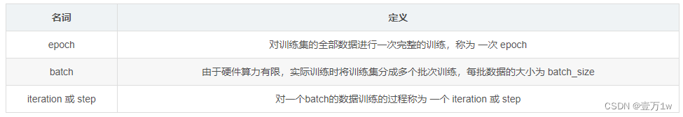
以本demo为例,训练集一共有50000个样本,batch_size=50,那么完整的训练一次样本:iteration或step=1000,epoch=1
net = LeNet()						  				# 定义训练的网络模型
loss_function = nn.CrossEntropyLoss() 				# 定义损失函数为交叉熵损失函数
optimizer = optim.Adam(net.parameters(), lr=0.001)  # 定义优化器(训练参数,学习率)

for epoch in range(5):  # 一个epoch即对整个训练集进行一次训练
    running_loss = 0.0
    time_start = time.perf_counter()

    for step, data in enumerate(train_loader, start=0):   # 遍历训练集,step从0开始计算
        inputs, labels = data 	# 获取训练集的图像和标签
        optimizer.zero_grad()   # 清除历史梯度

        # forward + backward + optimize
        outputs = net(inputs)  				  # 正向传播
        loss = loss_function(outputs, labels) # 计算损失
        loss.backward() 					  # 反向传播
        optimizer.step() 					  # 优化器更新参数

        # 打印耗时、损失、准确率等数据
        running_loss += loss.item()
        if step % 1000 == 999:    # print every 1000 mini-batches,每1000步打印一次
            with torch.no_grad(): # 在以下步骤中(验证过程中)不用计算每个节点的损失梯度,防止内存占用
                outputs = net(test_image) 				 # 测试集传入网络(test_batch_size=10000),output维度为[10000,10]
                predict_y = torch.max(outputs, dim=1)[1] # 以output中值最大位置对应的索引(标签)作为预测输出
                accuracy = (predict_y == test_label).sum().item() / test_label.size(0)

                print('[%d, %5d] train_loss: %.3f test_accuracy: %.3f' %  # 打印epoch,step,loss,accuracy
                      (epoch + 1, step + 1, running_loss / 500, accuracy))

                print('%f s' % (time.perf_counter() - time_start))        # 打印耗时
                running_loss = 0.0

print('Finished Training')

# 保存训练得到的参数
save_path = './Lenet.pth'
torch.save(net.state_dict(), save_path)
打印信息如下:
[1,  1000] train_loss: 1.537  test_accuracy: 0.541
35.345407 s
[2,  1000] train_loss: 1.198  test_accuracy: 0.605
40.532376 s
[3,  1000] train_loss: 1.048  test_accuracy: 0.641
44.144097 s
[4,  1000] train_loss: 0.954  test_accuracy: 0.647
41.313228 s
[5,  1000] train_loss: 0.882  test_accuracy: 0.662
41.860646 s
Finished Training
2.3 使用GPU/CPU训练
使用下面语句可以在有GPU时使用GPU,无GPU时使用CPU进行训练
device = torch.device("cuda" if torch.cuda.is_available() else "cpu")
print(device)
也可以直接指定
device = torch.device("cuda")
# 或者
# device = torch.device("cpu")
对应的,需要用to()函数来将Tensor在CPU和GPU之间相互移动,分配到指定的device中计算
net = LeNet()
net.to(device) # 将网络分配到指定的device中
loss_function = nn.CrossEntropyLoss()
optimizer = optim.Adam(net.parameters(), lr=0.001)

for epoch in range(5):

    running_loss = 0.0
    time_start = time.perf_counter()
    for step, data in enumerate(train_loader, start=0):
        inputs, labels = data
        optimizer.zero_grad()
        outputs = net(inputs.to(device))				  # 将inputs分配到指定的device中
        loss = loss_function(outputs, labels.to(device))  # 将labels分配到指定的device中
        loss.backward()
        optimizer.step()
        running_loss += loss.item()
        if step % 1000 == 999:
            with torch.no_grad():
                outputs = net(test_image.to(device)) # 将test_image分配到指定的device中
                predict_y = torch.max(outputs, dim=1)[1]
                accuracy = (predict_y == test_label.to(device)).sum().item() / test_label.size(0) # 将test_label分配到指定的device中

                print('[%d, %5d] train_loss: %.3f test_accuracy: %.3f' %
                      (epoch + 1, step + 1, running_loss / 1000, accuracy))

                print('%f s' % (time.perf_counter() - time_start))
                running_loss = 0.0

print('Finished Training')

save_path = './Lenet.pth'
torch.save(net.state_dict(), save_path)
打印信息如下:
cuda
[1,  1000] train_loss: 1.569  test_accuracy: 0.527
18.727597 s
[2,  1000] train_loss: 1.235  test_accuracy: 0.595
17.367685 s
[3,  1000] train_loss: 1.076  test_accuracy: 0.623
17.654908 s
[4,  1000] train_loss: 0.984  test_accuracy: 0.639
17.861825 s
[5,  1000] train_loss: 0.917  test_accuracy: 0.649
17.733115 s
Finished Training
可以看到,用GPU训练时,速度提升明显,耗时缩小。
3. predict.py
# 导入包
import torch
import torchvision.transforms as transforms
from PIL import Image
from model import LeNet

# 数据预处理
transform = transforms.Compose(
    [transforms.Resize((32, 32)), # 首先需resize成跟训练集图像一样的大小
     transforms.ToTensor(),
     transforms.Normalize((0.5, 0.5, 0.5), (0.5, 0.5, 0.5))])

# 导入要测试的图像(自己找的,不在数据集中),放在源文件目录下
im = Image.open('horse.jpg')
im = transform(im)  # [C, H, W]
im = torch.unsqueeze(im, dim=0)  # 对数据增加一个新维度,因为tensor的参数是[batch, channel, height, width]

# 实例化网络,加载训练好的模型参数
net = LeNet()
net.load_state_dict(torch.load('Lenet.pth'))

# 预测
classes = ('plane', 'car', 'bird', 'cat',
           'deer', 'dog', 'frog', 'horse', 'ship', 'truck')
with torch.no_grad():
    outputs = net(im)
    predict = torch.max(outputs, dim=1)[1].data.numpy()
print(classes[int(predict)])
输出即为预测的标签。
其实预测结果也可以用 softmax 表示,输出10个概率:
with torch.no_grad():
    outputs = net(im)
    predict = torch.softmax(outputs, dim=1)
print(predict)
输出结果中最大概率值对应的索引即为 预测标签 的索引。
tensor([[2.2782e-06, 2.1008e-07, 1.0098e-04, 9.5135e-05, 9.3220e-04, 2.1398e-04,
         3.2954e-08, 9.9865e-01, 2.8895e-08, 2.8820e-07]])
边栏推荐
猜你喜欢

随机推荐
数据库的基本语法(其一)
CVPR2020: Seeing Through Fog Without Seeing Fog
四大组件之一BroadCast(其一)
MPLS 实验
【mysql】查询不区分大小写(用户密码登录不区分大小写)
AI智能图像识别的工作原理及行业应用
NodeRed系列—nodered安装及基本操作
微信小程序部分功能细节
GBase 8s共享内存中的常驻内存段
Robust 3D Object Detection in Cold Weather Conditions
LiDAR Snowfall Simulation for Robust 3D Object Detection
【转载】图表:数读2022年上半年国民经济
mysq基础语句+高级操作(学这篇就够了)
Thread Handler
windows下的redis安装及密码修改
【uniapp】跨端开发问题记录
Maykel Studio - Django Web Application Framework + MySQL Database Second Training
Toward a Unified Model
Redis持久化方案RDB详解
华为adb wifi调试断线问题解决