当前位置:网站首页>Don't bother tensorflow learning notes (10-12) -- Constructing a simple neural network and its visualization
Don't bother tensorflow learning notes (10-12) -- Constructing a simple neural network and its visualization
2022-04-23 20:14:00 【Trabecular trying to write code】
This note is based on Mo fan python Of Tensorflow course
Personally, I don't think the video tutorial of don't bother God is suitable for Xiaobai with zero Foundation , If it's Xiaobai, you can watch the videos of Li Hongyi or Wu Enda first or read directly . Don't bother the great God's tutorial, which is suitable for in-depth learning. You already have some theoretical knowledge , But students who lack code foundation ( For example, I ), Basically, don't bother to write the code again , Xiaobian has been right tensorflow Have a certain understanding of the application of , Also mastered some training skills of neural network .
The following corresponds to... In the video Tensorflow course (10)(11)(12), Xiaobian will record according to Mo fan's explanation and my own understanding .
One 、 Understanding the structure of neural networks
The purpose of this tutorial is to build the simplest neural network . The simplest neural network structure is that it contains only one input layer( Input layer ), One hidden layer, One output layer( Output layer ). Each layer contains neurons , except hidden layer The number of neurons is a super parameter , The number of neurons in input layer and output layer is closely related to input data and output data . for instance , The input data defined in the program is :x_data, Then the number of neurons in the input layer is the same as that of the input data data The number of is related to . Be careful ! Not with data The number of samples in ! The same goes for the output layer .
The number of neurons in the hidden layer should not be too many , Because deep learning should be reflected in the number of hidden layers , If there are too many neurons in one layer , Then it should be breadth learning . Also important is the number of hidden layers , Blindly adding hidden layers will lead to over fitting( Over fitting ) problem . So the design of hidden layer is a knowledge based on experience .
Two 、 Code details
1、 Add layer creation def add_layer()
def add_layer(inputs,in_size,out_size,activation_function=None):
    Weights=tf.Variable(tf.random_normal([in_size,out_size]))
    biases=tf.Variable(tf.zeros([1,out_size])+0.1)
    Wx_plus_b=tf.matmul(inputs,Weights)+biases
    if activation_function is None:
        outputs=Wx_plus_b
    else:
        outputs=activation_function(Wx_plus_b)

    return outputs
First define the function as the input layer for subsequent creation , The basis of hidden layer and output layer . What needs special attention here , In many cases, we are defining bias Time will make bias=0, But I don't want to bias=0, So in the biases Add after 0.1, Guaranteed not to be zero .
Yes activation_function The judgment of the : In the connection between input layer and hidden layer , We need to use activation_function Convert the data into a non-linear form , But in the connection between the hidden layer and the output layer , We no longer need to activate the function . Because there is a judgment , When you don't need to activate a function , Direct output Wx_plus_b; When needed , will Wx_plus_b Output after activating the function .
2、 Data import and neural network establishment
x_data=np.linspace(-1,1,300)[:,np.newaxis]
noise=np.random.normal(0,0.05,x_data.shape)
y_data=np.square(x_data)-0.5+noise

xs=tf.placeholder(tf.float32,[None,1])
ys=tf.placeholder(tf.float32,[None,1])
l1=add_layer(xs,1,10,activation_function=tf.nn.relu)#l1 is an input layer
#activation function is a relu function
prediction=add_layer(l1,10,1,activation_function=None)#prediction is an hidden layer

loss=tf.reduce_mean(tf.reduce_sum(tf.square(ys-prediction),reduction_indices=[1]))
#loss function is based on MSE(mean square error)
train_step=tf.train.GradientDescentOptimizer(0.1).minimize(loss)

init=tf.global_variables_initializer() #initialize all variables
sess=tf.Session()
sess.run(init) #very important
We use noise to import data (noise). use noise To get y_data Not exactly according to the direction of univariate quadratic function ,y_data The results must be random , So in bias Added... To the location noise, Got y-x The image is shown below :

Here we use tensorflow Medium placeholder function .placeholder() Functions are constructed in neural networks graph In the model , The data to be input is not passed into the model at this time , It just allocates the necessary memory . Etc session, In conversation , Run the model by feed_dict() Function passes data to the placeholder .
use placeholder Is that , You can customize the amount of incoming data . In the training of deep learning , Generally, the whole data set will not be trained directly , For example, random gradient descent (Stochastic Gradient Descent) Is to take mini batch Train the data in a way .
3、 Neural network training visualization
In this program, visualization uses matplotlib library , And dynamically display the training results . But don't bother with the code directly in jupyter notebook It will happen when running on. Only function images can be displayed , The problem of not displaying images dynamically . stay youtube In the comments under Mofan's video , Many small partners also reflect that whether it is IDLE still terminal Or other compilation environments , Add... To the front in time %matplotlib inline It can't achieve the expected effect . Small series search method , Several methods can be found in jupyter notebook Method of dynamic display on . But this method needs to install Qt,jupyter Will use Qt As drawing backend .
The code is as follows :
%matplotlib # Declare when importing the library


fig=plt.figure()
ax=fig.add_subplot(1,1,1)
ax.scatter(x_data,y_data)
plt.ion()
plt.show()

for i in range(2000):
    sess.run(train_step,feed_dict={xs:x_data,ys:y_data})
    if i%50==0:
         try:
                plt.pause(0.5)
        except Exception:
            pass

        try:
            ax.lines.remove(lines[0])
            plt.show()
        except Exception as e:
            pass

        prediction_value=sess.run(prediction,feed_dict={xs:x_data})
        lines=ax.plot(x_data,prediction_value,'r-',lw=10)

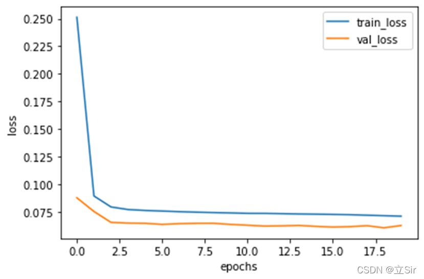
This is the training effect after adding dynamic images , The red curve is the curve trained by computer , The blue dot area is x、y The area of the true value of the point . You can see that after computer training , We can get a curve that roughly matches the regional trend .
That's the whole content of the tutorial , If you have any questions, please communicate in the comment area !
版权声明
本文为[Trabecular trying to write code]所创,转载请带上原文链接,感谢
https://yzsam.com/2022/04/202204210555381778.html
边栏推荐
- Why is the hexadecimal printf output of C language sometimes with 0xff and sometimes not
- nc基础用法3
- MySQL数据库 - 单表查询(三)
- R language uses the preprocess function of caret package for data preprocessing: BoxCox transform all data columns (convert non normal distribution data columns to normal distribution data and can not
- MySQL数据库 - 单表查询(一)
- 【数值预测案例】(3) LSTM 时间序列电量预测,附Tensorflow完整代码
- Inject Autowired fields into ordinary beans
- aqs的学习
- An error is reported when sqoop imports data from Mysql to HDFS: sqlexception in nextkeyvalue
- Mysql database - basic operation of database and table (II)
猜你喜欢
山东大学软件学院项目实训-创新实训-网络安全靶场实验平台(六)

Project training of Software College of Shandong University - Innovation Training - network security shooting range experimental platform (V)
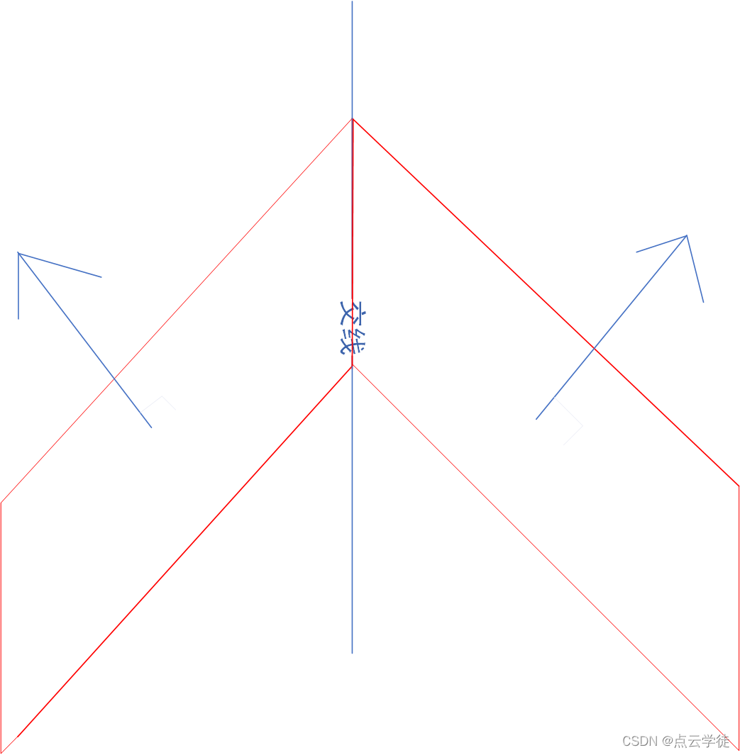
Computing the intersection of two planes in PCL point cloud processing (51)
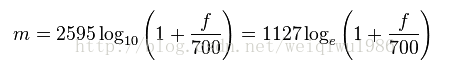
Mfcc: Mel frequency cepstrum coefficient calculation of perceived frequency and actual frequency conversion
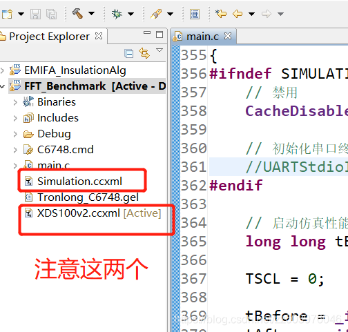
C6748 software simulation and hardware test - with detailed FFT hardware measurement time

DTMF dual tone multi frequency signal simulation demonstration system
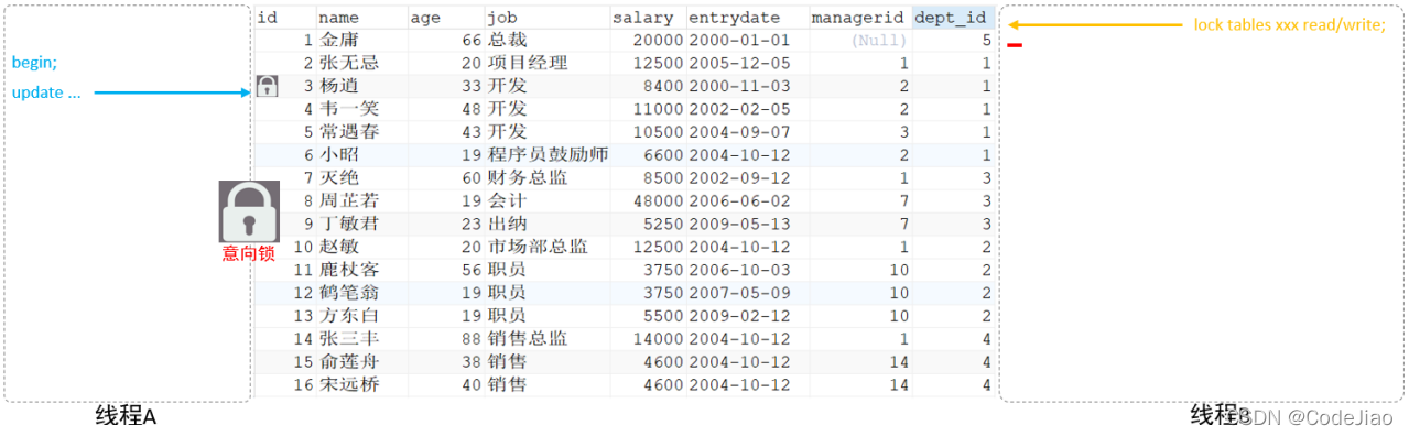
MySQL 进阶 锁 -- MySQL锁概述、MySQL锁的分类:全局锁(数据备份)、表级锁(表共享读锁、表独占写锁、元数据锁、意向锁)、行级锁(行锁、间隙锁、临键锁)
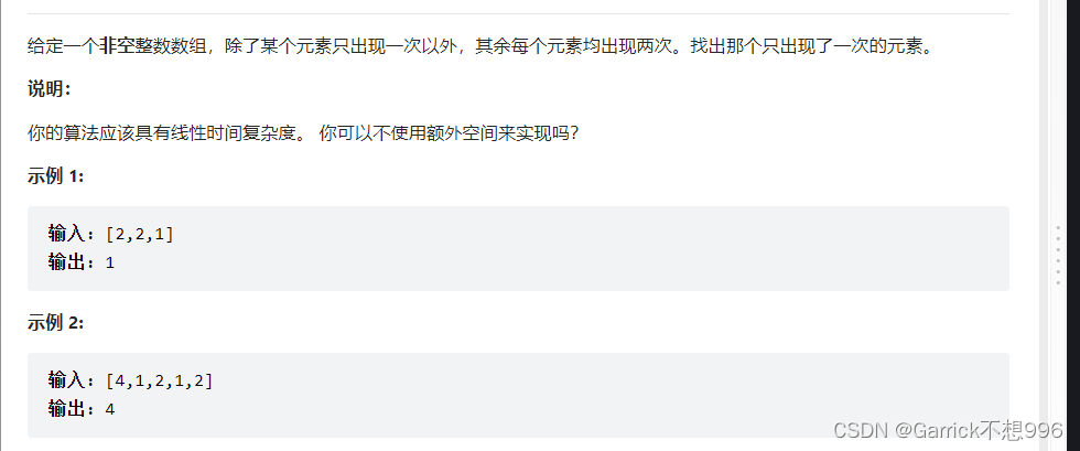
LeetCode异或运算

基于pytorch搭建GoogleNet神经网络用于花类识别
【数值预测案例】(3) LSTM 时间序列电量预测,附Tensorflow完整代码
随机推荐
基于pytorch搭建GoogleNet神经网络用于花类识别
STM32基础知识
PCL点云处理之直线与平面的交点计算(五十三)
Tencent Qiu Dongyang: techniques and ways of accelerating deep model reasoning
PCA based geometric feature calculation of PCL point cloud processing (52)
NC basic usage 3
Kubernetes getting started to proficient - install openelb on kubernetes
本地调用feign接口报404
考研英语唐叔的语法课笔记
Notes of Tang Shu's grammar class in postgraduate entrance examination English
R language uses the preprocess function of caret package for data preprocessing: BoxCox transform all data columns (convert non normal distribution data columns to normal distribution data and can not
selenium. common. exceptions. WebDriverException: Message: ‘chromedriver‘ executable needs to be in PAT
Cadence Orcad Capture CIS更换元器件之Link Database 功能介绍图文教程及视频演示
NC basic usage 4
Kubernetes introduction to mastery - ktconnect (full name: kubernetes toolkit connect) is a small tool based on kubernetes environment to improve the efficiency of local test joint debugging.
Understanding various team patterns in scrum patterns
Azkaban recompile, solve: could not connect to SMTP host: SMTP 163.com, port: 465 [January 10, 2022]
【数值预测案例】(3) LSTM 时间序列电量预测,附Tensorflow完整代码
MySQL数据库 - 单表查询(三)
Use test of FFT and IFFT library functions of TI DSP