当前位置:网站首页>Machine learning theory (8): model integration ensemble learning
Machine learning theory (8): model integration ensemble learning
2022-04-23 18:34:00 【Flying warm】
List of articles
The idea of integrated learning
- By constructing multiple base classifiers (base classifier) The classification results of these base classifiers are integrated to get the final prediction results

- The method of model integration is based on the following intuition :
- The sum decision of multiple models is better than that of a single model
- The results of multiple weak classifiers are at least the same as that of one strong classifier
- The results of multiple strong classifiers are at least the same as that of one base classifier
Must the results of multiple classifiers be good
- C 1 , C 2 , C 3 C_1,C_2,C_3 C1,C2,C3 They represent 3 Base classifiers , C ∗ C^* C∗ It represents the final result of the combination of three classifiers :

- Experimental results show that the integrated result is not necessarily better than a single classifier
When model integration is effective
- Base classifiers don't make the same mistakes
- Each base classifier has reasonable accuracy
How to construct a base classifier
- Through the division of training examples, multiple different base classifiers are generated : Sample the sample instance multiple times , A base classifier is generated for each sampling
- Multiple different base classifiers are generated through the feature division of training examples : Divide the feature set into multiple subsets , Multiple base classifiers are trained by samples with different feature subsets
- Multiple different base classifiers are generated through algorithm adjustment : Given an algorithm , Then, multiple training bases are generated according to different classifier parameters .
How to classify by base classifier
- The most common method of classification by multiple base classifiers is laws and regulations governing balloting
- For discrete output results , The final classification result can be obtained by counting , For example, a binary dataset ,label=0/1, constructed 5 Base classifiers , For a sample with three base classifiers, the output result is 1, Two are 0 So at this point , In sum, the result should be 1
- For continuous output results , Their results can be averaged to get the final results of multiple base classifiers
The generalization error of the model
- Bias( bias ): Measure the tendency of a classifier to make false predictions
- Variance( Variability ): Measure the deviation of a classifier's prediction results
- If a model has smaller bias and variance It means that the generalization performance of this model is very good .
Classifier integration method
Bagging Bagging
- The core idea : More data should have better performance ; So how to generate more data through fixed data sets ?
- Multiple different data sets are generated by random sampling and replacement
- The original data set is randomly sampled with put back N N N Time , Got it N N N Data sets , For these data sets, a total of N N N Different base classifiers
- For this N N N A classifier , Let them use the voting method to decide the final classification result
- But there's a problem with bagging , That is, some samples may never be used . because N N N Samples , The probability of each sample being taken is 1 N \frac{1}{N} N1 Then take a total of N N N The probability of not getting it is ( 1 − 1 N ) N (1-\frac{1}{N})^N (1−N1)N This value is in the N N N The limit value when it is very large ≈ 0.37 \approx0.37 ≈0.37
- Characteristics of bagging method :
- This is an integrated method based on sampling and voting (instance manipulation)
- Multiple independent base classifiers can be calculated synchronously and in parallel
- It can effectively overcome the noise in the data set
- In general, the result is much better than that of a single base classifier , However, there are also cases where the effect is worse than that of a single base classifier
Random forest method Random Forest
-
The single classifier on which the random forest depends is the decision tree , But this decision tree is slightly different from the previous decision tree
-
A single decision tree used in random forest only selects some features to establish the tree . In other words, the feature space used by the trees in the random forest is not all the feature space
- for example , Adopt a fixed proportion τ \tau τ To select the feature space size of each decision tree
- The establishment of each tree in a random forest is simpler and faster than a single decision tree ; But this method increases the accuracy of the model variance
-
Each tree in the random forest uses a different training set (using different bagged training dataset)
-
Finally, the final result is obtained by voting .

-
The idea of this operation is : Minimize the association between any two trees
-
Hyperparameters of random forests :
- The number of trees in the forest B B B
- The size of each feature subset , As the size increases , The ability and relevance of classifiers have increased ( ⌊ l o g 2 ∣ F ∣ + 1 ⌋ \lfloor log_2|F|+1\rfloor ⌊log2∣F∣+1⌋) Because each tree in a random forest uses more features , The higher the coincidence with the characteristics of other trees in the forest , The greater the similarity of random numbers
- Interpretability : The logic behind single instance prediction can be determined by multiple random trees
-
The characteristics of random forest :
- The forest is very random , Can be built efficiently
- Can be carried out in parallel
- Strong robustness to over fitting
- Interpretability is sacrificed in part , Because the features of each tree are randomly selected from the feature set
Evolution method Boosting
-
boosting The method mainly focuses on difficult samples
-
boosting Weak learners can be promoted to strong learners , Its operation mechanism is :
- A base learner is trained from the initial training set ; At this time, each sample instance All of the weights 1 N \frac{1}{N} N1
- Every iteration The weight of the training set samples will be adjusted according to the prediction results of the previous round
- Training a new basic learner based on the adjusted training set
- Repeat , Until the number of base learners reaches the value set at the beginning T T T
- take T T T A base learner uses a weighted voting method (weighted voting ) Combine
-
about boosting Method , There are two problems to be solved :
- How should each round of learning change the probability distribution of data
- How to combine various base classifiers


AdaBoost
- adaptive boosting Adaptive enhancement algorithm ; Is a sequential integration method ( Random forest and Bagging All belong to parallel integration algorithms )
- AdaBoost The basic idea of :
- Yes T T T Base classifiers : C 1 , C 2 , . . . , C i , . . . , C T C_1,C_2,...,C_i,...,C_T C1,C2,...,Ci,...,CT
- The training set is expressed as { x j , y j ∣ j = 1 , 2 , . . , N } \{x_j,y_j|j=1,2,..,N\} { xj,yj∣j=1,2,..,N}
- Initialize the weight of each sample to 1 N \frac{1}{N} N1, namely : { w j ( 1 ) = 1 N ∣ j = 1 , 2 , . . . , N } \{w_j^{(1)}=\frac{1}{N}|j=1,2,...,N\} { wj(1)=N1∣j=1,2,...,N}
At every iteration i i i in , Follow the steps below :
- Calculate the error rate error rate ϵ i = Σ j = 1 N w j δ ( C i ( x j ) ≠ y j ) \epsilon_i=\Sigma_{j=1}^Nw_j\delta(C_i(x_j)\neq y_j) ϵi=Σj=1Nwjδ(Ci(xj)=yj)
- δ ( ⋅ ) \delta(\cdot) δ(⋅) It's a indicator function , When the condition of the function is satisfied, the value of the function is 1 1 1; namely , When the weak classifier C i C_i Ci On the sample x j x_j xj If the classification is wrong, it will accumulate w j w_j wj
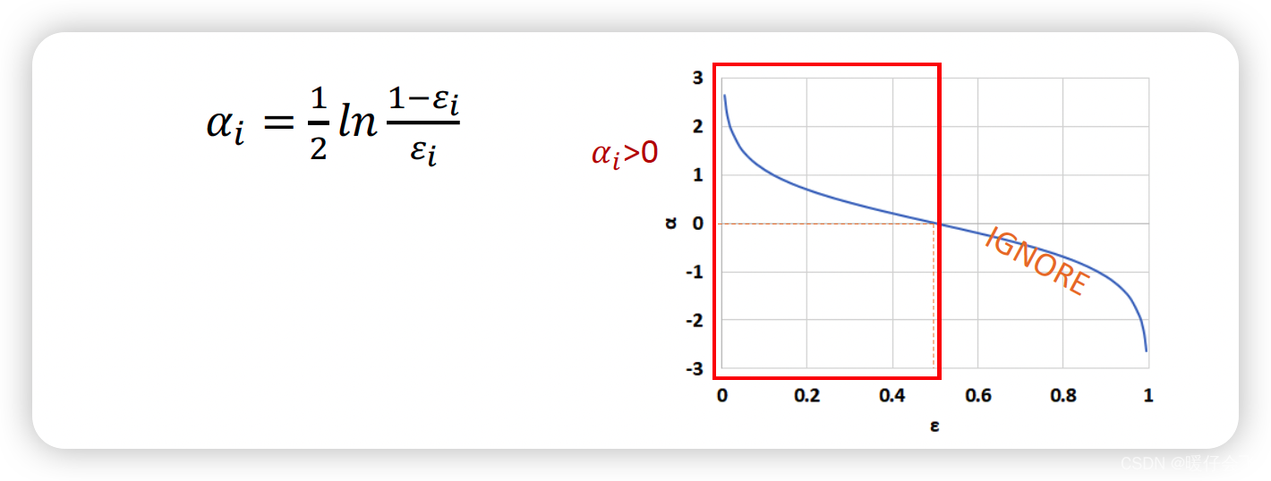
- Use ϵ i \epsilon_i ϵi To calculate each base classifier C i C_i Ci The importance of ( Assign weight to this base classifier α i \alpha_i αi) α i = 1 2 l n 1 − ϵ i ϵ i \alpha_i=\frac{1}{2}ln\frac{1-\epsilon_i}{\epsilon_i} αi=21lnϵi1−ϵi
- It can also be seen from this formula , When C i C_i Ci The larger the sample size that is wrong , Got ϵ i \epsilon_i ϵi The greater the , Corresponding α i \alpha_i αi The smaller ( The closer the 0 0 0 )
- according to α i \alpha_i αi To update Of each sample Weight parameters , For the sake of i + 1 i+1 i+1 individual iteration To prepare for :
- sample j j j The weight of is determined by w j ( i ) w_j^{(i)} wj(i) become w j ( i + 1 ) w_j^{(i+1)} wj(i+1) What happens in this process is : If this sample is in the i i i individual iteration Was judged right , His weight will be in the original w j ( i ) w_j^{(i)} wj(i) Multiply by e − α i e^{-\alpha_i} e−αi; Based on the above knowledge α i > 0 \alpha_i>0 αi>0 therefore − α i < 0 -\alpha_i<0 −αi<0 So according to the formula, we can know , Those samples predicted incorrectly by the classifier will have a large weight ; The sample with the correct prediction will have a smaller weight ;
- Z ( i ) Z^{(i)} Z(i) It's a normalization term , In order to ensure that the sum of all weights is 1 1 1
- In the end, all the C i C_i Ci Integration by weight
- Continue to complete from i = 2 , . . . , T i=2,...,T i=2,...,T Iterative process of , But when ϵ i > 0.5 \epsilon_i>0.5 ϵi>0.5 You need to reinitialize the weight of the sample
Finally, the integration model is used to classify the formula : C ∗ ( x ) = a r g m a x y Σ i = 1 T α i δ ( C i ( x ) = y ) C^*(x)=argmax_y\Sigma_{i=1}^T \alpha_i\delta(C_i(x)=y) C∗(x)=argmaxyΣi=1Tαiδ(Ci(x)=y)
- This formula probably means : For example, we have now got 3 3 3 Base classifiers , Their weights are 0.3 , 0.2 , 0.1 0.3, 0.2, 0.1 0.3,0.2,0.1 So the whole ensemble classifier can be expressed as C ( x ) = Σ i = 1 T α i C i ( x ) = 0.3 C 1 ( x ) + 0.2 C 2 ( x ) + 0.1 C 3 ( x ) C(x)=\Sigma_{i=1}^T \alpha_iC_i(x)=0.3C_1(x)+0.2C_2(x) +0.1C_3(x) C(x)=Σi=1TαiCi(x)=0.3C1(x)+0.2C2(x)+0.1C3(x) If there are only 0 , 1 0,1 0,1 Then the final C ( x ) C(x) C(x) about 0 0 0 Is the value of the larger or for 1 1 1 The value of is big .
As long as each base classifier is better than random prediction , Finally, many models will converge to one


- Boosting Characteristics of the integration method :
- His base classifier is a decision tree or OneR Method
- The mathematical process is complicated , But the computational overhead is small ; The whole process is based on iterative sampling process and weighted voting (voting) On
- The residual information is fitted continuously through iteration , Finally, ensure the accuracy of the model
- Than bagging The computational cost of the method is higher
- In practical applications ,boosting The method has a slight tendency of over fitting ( But it's not serious )
- May be the best word classifier (gradient boosting)
Bagging / Random Forest as well as Boosting contrast

Stacking Stacking
- Use a variety of algorithms , These algorithms have different bias
In the base classifier (level-0 model) Train a meta classifier on the output of (meta-classifier) Also called level-1 model
- Know which classifiers are reliable , And combine the output of the base classifier
- Use cross validation to reduce bias
-
Level-0: Base classifier
- Given a dataset ( X , y ) (X,y) (X,y)
- It can be SVM, Naive Bayes, DT etc.
-
Level-1: Ensemble classifiers
- stay Level-0 A new classifier is constructed based on the classifier attributes
- Every Level-0 The predicted output of the classifier will be added as a new attributes; If there is M M M individual level-0 The separator will eventually add M M M individual attributes
- Delete or keep the original data X X X
- Consider other available data (NB Probability score ,SVM The weight )
- Training meta-classifier To make the final prediction
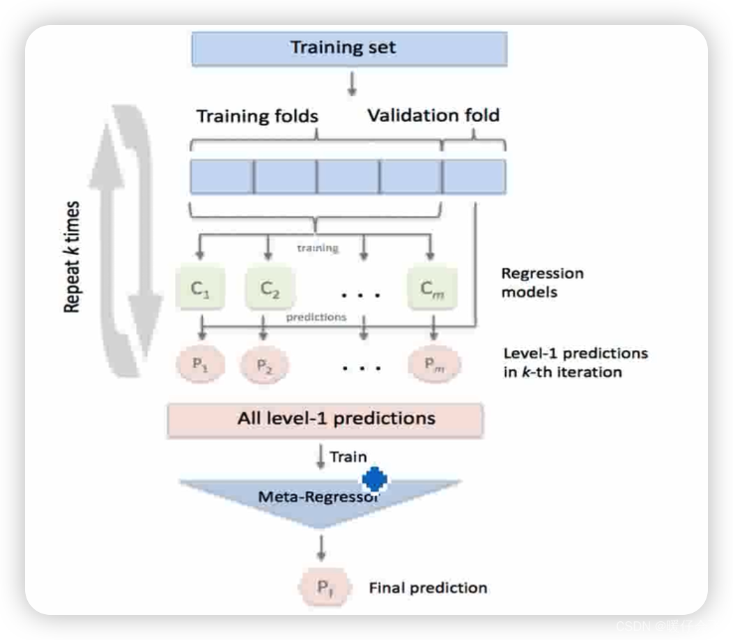
Visualize this stacking This process
- Firstly, the original data is divided into training set and verification set , For example, here 4 For training ,1 For testing
- Use these data for training ( X t r a i n , y t r a i n ) (X_{train},y_{train}) (Xtrain,ytrain) To train m m m Base classifiers C 1 , . . . , C m C_1,...,C_m C1,...,Cm, Test each classifier data set ( X t e s t , y t e s t ) (X_{test},y_{test}) (Xtest,ytest) Conduct predict Get the prediction P 1 , . . . , P m P_1,...,P_m P1,...,Pm, Then compare the predicted results with the label of the original Tester y t e s t y_{test} ytest Make a new training set ( X n e w , y t e s t ) (X_{new},y_{test}) (Xnew,ytest), among X n e w = { P 1 , . . . , P m } X_{new}=\{P_1,...,P_m\} Xnew={ P1,...,Pm} To train level-1 The integration model of .
- stacking Characteristics of the method :
- Combine a variety of different classifiers
- The mathematical expression is simple , But the actual operation consumes computing resources
- Usually compared with base classifier ,stacking The results are generally better than the best base classifier
版权声明
本文为[Flying warm]所创,转载请带上原文链接,感谢
https://yzsam.com/2022/04/202204231826143956.html
边栏推荐
- 机器学习实战 -朴素贝叶斯
- Stm32mp157 wm8960 audio driver debugging notes
- os_authent_prefix
- Robocode Tutorial 4 - robocode's game physics
- 14个py小游戏源代码分享第二弹
- On iptables
- Test questions of daily safety network (February 2024)
- 机器学习理论之(7):核函数 Kernels —— 一种帮助 SVM 实现非线性化决策边界的方式
- Solution to Chinese garbled code after reg file is imported into the registry
- 【ACM】509. 斐波那契数(dp五部曲)
猜你喜欢
listener. log

根据快递单号查询物流查询更新量
The vivado project corresponding to the board is generated by TCL script

How to virtualize the video frame and background is realized in a few simple steps
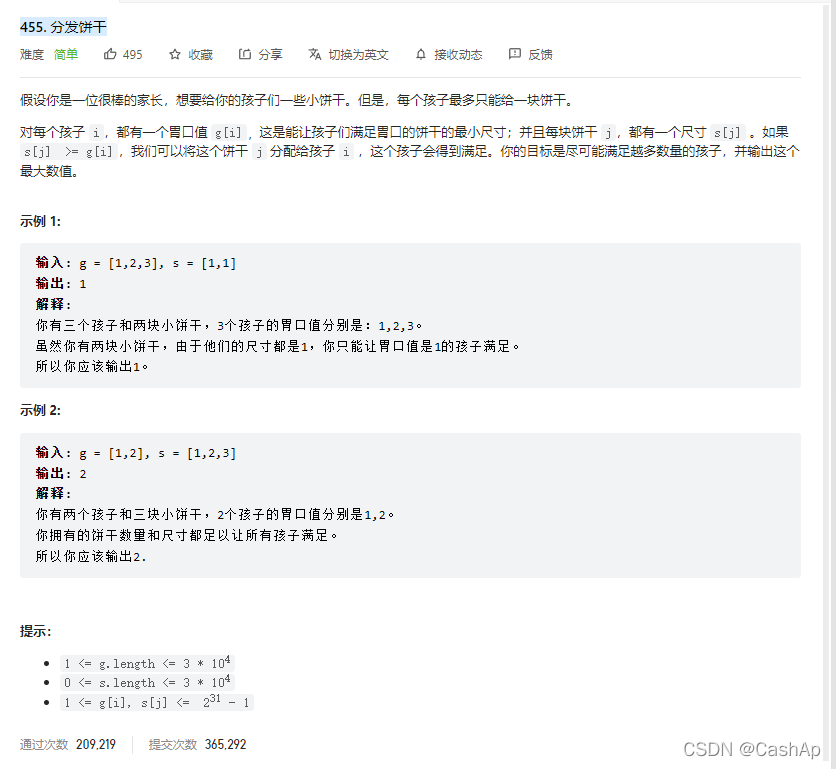
【ACM】455. 分发饼干(1. 大饼干优先喂给大胃口;2. 遍历两个数组可以只用一个for循环(用下标索引--来遍历另一个数组))
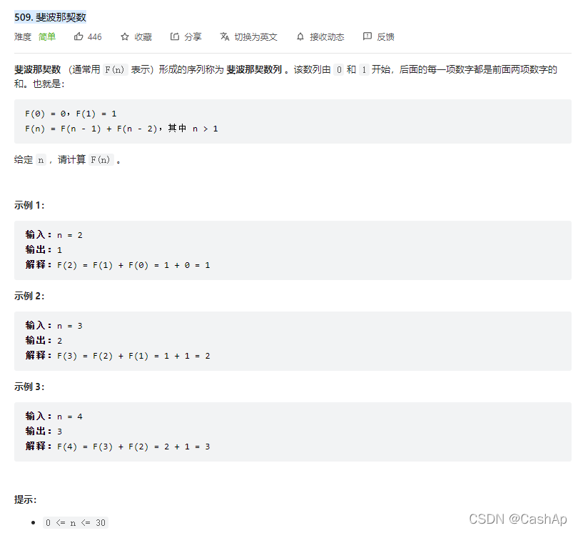
【ACM】509. Fibonacci number (DP Trilogy)
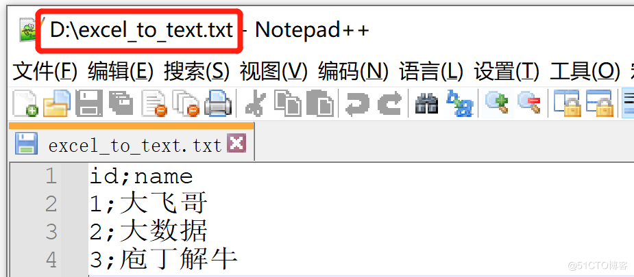
kettle庖丁解牛第17篇之文本文件输出

Use stm32cube MX / stm32cube ide to generate FatFs code and operate SPI flash

Solution to Chinese garbled code after reg file is imported into the registry
【ACM】455. Distribute Biscuits (1. Give priority to big biscuits to big appetite; 2. Traverse two arrays with only one for loop (use subscript index -- to traverse another array))
随机推荐
CISSP certified daily knowledge points (April 12, 2022)
【ACM】376. 摆动序列
纠结
Test questions of daily safety network (February 2024)
Creation and use of QT dynamic link library
Daily network security certification test questions (April 13, 2022)
Using transmittablethreadlocal to realize parameter cross thread transmission
Can filter
软件测试总结
WIN1 remote "this may be due to credssp encryption Oracle correction" solution
How to restore MySQL database after win10 system is reinstalled (mysql-8.0.26-winx64. Zip)
Daily CISSP certification common mistakes (April 19, 2022)
【ACM】70. 爬楼梯
JD-FreeFuck 京东薅羊毛控制面板 后台命令执行漏洞
线上怎么确定期货账户安全的?
CANopen STM32 transplantation
CISSP certified daily knowledge points (April 19, 2022)
Quantexa CDI(场景决策智能)Syneo平台介绍
In win10 system, all programs run as administrator by default
机器学习理论之(8):模型集成 Ensemble Learning