当前位置:网站首页>Matlab tips (6) comparison of seven filtering methods
Matlab tips (6) comparison of seven filtering methods
2022-04-23 18:10:00 【mozun2020】
MATLAB Tips (6) Comparison of seven filtering methods
Preface
MATLAB Learning about image processing is very friendly , You can start from scratch , There are many encapsulated functions that can be called directly for basic image processing , This series of articles is mainly to introduce some of you in MATLAB Some concept functions are commonly used in routine demonstration !
The seven filtering methods are Butterworth low-pass filtering 、FIR Low pass filtering 、 Moving average filtering 、 median filtering 、 Wiener filtering 、 Adaptive filtering 、 Wavelet filtering . Different filtering methods , There will be different emphasis on all kinds of noise , The treatment effect is also different . In this experiment, the filtering effect of adaptive filtering method is better .
One . MATLAB Simulation
%****************************************************************************************
%
% Create two signals Mix_Signal_1 And signals Mix_Signal_2
%
%***************************************************************************************
clc;clear;close;
Fs = 1000; % Sampling rate
N = 1000; % Number of sampling points
n = 0:N-1;
t = 0:1/Fs:1-1/Fs; % The time series
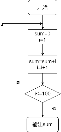
Signal_Original_1 =sin(2*pi*10*t)+sin(2*pi*20*t)+sin(2*pi*30*t);
Noise_White_1 = [0.3*randn(1,500), rand(1,500)]; % front 500 Point Gaussian partial white noise , after 500 Point uniformly distributed white noise
Mix_Signal_1 = Signal_Original_1 + Noise_White_1; % Constructed mixed signal
Signal_Original_2 = [zeros(1,100), 20*ones(1,20), -2*ones(1,30), 5*ones(1,80), -5*ones(1,30), 9*ones(1,140), -4*ones(1,40), 3*ones(1,220), 12*ones(1,100), 5*ones(1,20), 25*ones(1,30), 7 *ones(1,190)];
Noise_White_2 = 0.5*randn(1,1000); % white Gaussian noise
Mix_Signal_2 = Signal_Original_2 + Noise_White_2; % Constructed mixed signal
%****************************************************************************************
%
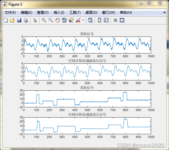
% The signal Mix_Signal_1 and Mix_Signal_2 Make Butterworth low-pass filtering respectively .
%
%***************************************************************************************
% Mixed signal Mix_Signal_1 Butterworth low pass filter
figure(1);
Wc=2*50/Fs; % Cut off frequency 50Hz
[b,a]=butter(4,Wc);
Signal_Filter=filter(b,a,Mix_Signal_1);
subplot(4,1,1); %Mix_Signal_1 The original signal
plot(Mix_Signal_1);
axis([0,1000,-4,4]);
title(' The original signal ');
subplot(4,1,2); %Mix_Signal_1 Low pass filtered signal
plot(Signal_Filter);
axis([0,1000,-4,4]);
title(' Butterworth low pass filtered signal ');
% Mixed signal Mix_Signal_2 Butterworth low pass filter
Wc=2*100/Fs; % Cut off frequency 100Hz
[b,a]=butter(4,Wc);
Signal_Filter=filter(b,a,Mix_Signal_2);
subplot(4,1,3); %Mix_Signal_2 The original signal
plot(Mix_Signal_2);
axis([0,1000,-10,30]);
title(' The original signal ');
subplot(4,1,4); %Mix_Signal_2 Low pass filtered signal
plot(Signal_Filter);
axis([0,1000,-10,30]);
title(' Butterworth low pass filtered signal ');
%****************************************************************************************
%
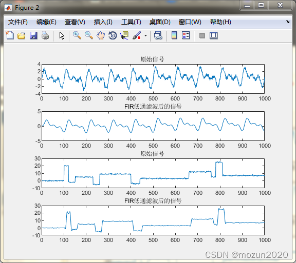
% The signal Mix_Signal_1 and Mix_Signal_2 Make separately FIR Low pass filtering .
%
%***************************************************************************************
% Mixed signal Mix_Signal_1 FIR Low pass filtering
figure(2);
F = [0:0.05:0.95];
A = [1 1 0 0 0 0 0 0 0 0 0 0 0 0 0 0 0 0 0 0] ;
b = firls(20,F,A);
Signal_Filter = filter(b,1,Mix_Signal_1);
subplot(4,1,1); %Mix_Signal_1 The original signal
plot(Mix_Signal_1);
axis([0,1000,-4,4]);
title(' The original signal ');
subplot(4,1,2); %Mix_Signal_1 FIR Low pass filtered signal
plot(Signal_Filter);
axis([0,1000,-5,5]);
title('FIR Low pass filtered signal ');
% Mixed signal Mix_Signal_2 FIR Low pass filtering
F = [0:0.05:0.95];
A = [1 1 1 1 1 0 0 0 0 0 0 0 0 0 0 0 0 0 0 0] ;
b = firls(20,F,A);
Signal_Filter = filter(b,1,Mix_Signal_2);
subplot(4,1,3); %Mix_Signal_2 The original signal
plot(Mix_Signal_2);
axis([0,1000,-10,30]);
title(' The original signal ');
subplot(4,1,4); %Mix_Signal_2 FIR Low pass filtered signal
plot(Signal_Filter);
axis([0,1000,-10,30]);
title('FIR Low pass filtered signal ');
%****************************************************************************************
%
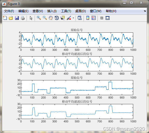
% The signal Mix_Signal_1 and Mix_Signal_2 Make moving average filtering respectively
%
%***************************************************************************************
% Mixed signal Mix_Signal_1 Moving average filtering
figure(3);
b = [1 1 1 1 1 1]/6;
Signal_Filter = filter(b,1,Mix_Signal_1);
subplot(4,1,1); %Mix_Signal_1 The original signal
plot(Mix_Signal_1);
axis([0,1000,-4,4]);
title(' The original signal ');
subplot(4,1,2); %Mix_Signal_1 Moving average filtered signal
plot(Signal_Filter);
axis([0,1000,-4,4]);
title(' Moving average filtered signal ');
% Mixed signal Mix_Signal_2 Moving average filtering
b = [1 1 1 1 1 1]/6;
Signal_Filter = filter(b,1,Mix_Signal_2);
subplot(4,1,3); %Mix_Signal_2 The original signal
plot(Mix_Signal_2);
axis([0,1000,-10,30]);
title(' The original signal ');
subplot(4,1,4); %Mix_Signal_2 Moving average filtered signal
plot(Signal_Filter);
axis([0,1000,-10,30]);
title(' Moving average filtered signal ');
%****************************************************************************************
%
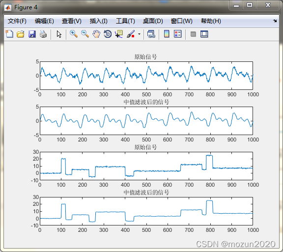
% The signal Mix_Signal_1 and Mix_Signal_2 Make median filtering respectively
%
%***************************************************************************************
% Mixed signal Mix_Signal_1 median filtering
figure(4);
Signal_Filter=medfilt1(Mix_Signal_1,10);
subplot(4,1,1); %Mix_Signal_1 The original signal
plot(Mix_Signal_1);
axis([0,1000,-5,5]);
title(' The original signal ');
subplot(4,1,2); %Mix_Signal_1 Median filtered signal
plot(Signal_Filter);
axis([0,1000,-5,5]);
title(' Median filtered signal ');
% Mixed signal Mix_Signal_2 median filtering
Signal_Filter=medfilt1(Mix_Signal_2,10);
subplot(4,1,3); %Mix_Signal_2 The original signal
plot(Mix_Signal_2);
axis([0,1000,-10,30]);
title(' The original signal ');
subplot(4,1,4); %Mix_Signal_2 Median filtered signal
plot(Signal_Filter);
axis([0,1000,-10,30]);
title(' Median filtered signal ');
%****************************************************************************************
%
% The signal Mix_Signal_1 and Mix_Signal_2 Make Wiener filtering respectively
%
%***************************************************************************************
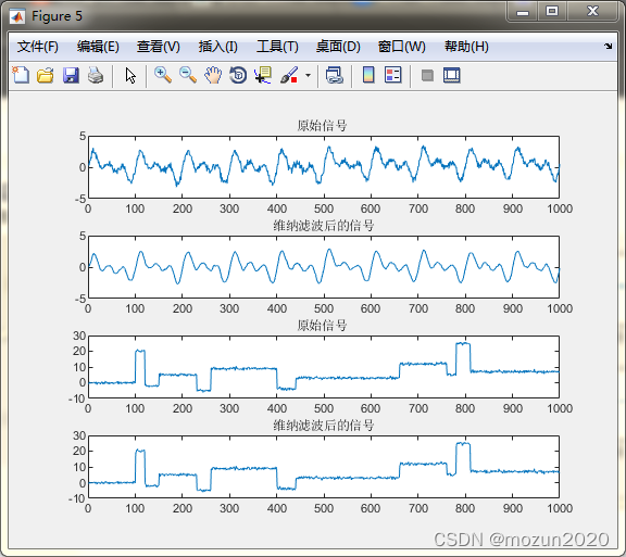
% Mixed signal Mix_Signal_1 Wiener filtering
figure(5);
Rxx=xcorr(Mix_Signal_1,Mix_Signal_1); % The autocorrelation function of the mixed signal is obtained
M=100; % Wiener filter order
for i=1:M % The autocorrelation matrix of the mixed signal is obtained
for j=1:M
rxx(i,j)=Rxx(abs(j-i)+N);
end
end
Rxy=xcorr(Mix_Signal_1,Signal_Original_1); % The cross-correlation function between the mixed signal and the original signal is obtained
for i=1:M
rxy(i)=Rxy(i+N-1);
end % The cross-correlation vector of the mixed signal and the original signal is obtained
h = inv(rxx)*rxy'; % Get what's involved wiener Filter coefficients
Signal_Filter=filter(h,1, Mix_Signal_1); % Pass the input signal through the Wiener filter
subplot(4,1,1); %Mix_Signal_1 The original signal
plot(Mix_Signal_1);
axis([0,1000,-5,5]);
title(' The original signal ');
subplot(4,1,2); %Mix_Signal_1 Wiener filtered signal
plot(Signal_Filter);
axis([0,1000,-5,5]);
title(' Wiener filtered signal ');
% Mixed signal Mix_Signal_2 Wiener filtering
Rxx=xcorr(Mix_Signal_2,Mix_Signal_2); % The autocorrelation function of the mixed signal is obtained
M=500; % Wiener filter order
for i=1:M % The autocorrelation matrix of the mixed signal is obtained
for j=1:M
rxx(i,j)=Rxx(abs(j-i)+N);
end
end
Rxy=xcorr(Mix_Signal_2,Signal_Original_2); % The cross-correlation function between the mixed signal and the original signal is obtained
for i=1:M
rxy(i)=Rxy(i+N-1);
end % The cross-correlation vector of the mixed signal and the original signal is obtained
h=inv(rxx)*rxy'; % Get what's involved wiener Filter coefficients
Signal_Filter=filter(h,1, Mix_Signal_2); % Pass the input signal through the Wiener filter
subplot(4,1,3); %Mix_Signal_2 The original signal
plot(Mix_Signal_2);
axis([0,1000,-10,30]);
title(' The original signal ');
subplot(4,1,4); %Mix_Signal_2 Wiener filtered signal
plot(Signal_Filter);
axis([0,1000,-10,30]);
title(' Wiener filtered signal ');
%****************************************************************************************
%
% The signal Mix_Signal_1 and Mix_Signal_2 Make adaptive filtering respectively
%
%***************************************************************************************
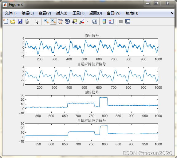
% Mixed signal Mix_Signal_1 Adaptive filtering
figure(6);
N=1000; % Input signal sampling points N
k=100; % Time domain tap LMS Algorithm filter order
u=0.001; % Step size factor
% Set the initial value
yn_1=zeros(1,N); %output signal
yn_1(1:k)=Mix_Signal_1(1:k); % The input signal SignalAddNoise Before k A value as output yn_1 Before k It's worth
w=zeros(1,k); % Set the initial value of tap weighting
e=zeros(1,N); % Error signal
% use LMS Iterative filtering algorithm
for i=(k+1):N
XN=Mix_Signal_1((i-k+1):(i));
yn_1(i)=w*XN';
e(i)=Signal_Original_1(i)-yn_1(i);
w=w+2*u*e(i)*XN;
end
subplot(4,1,1);
plot(Mix_Signal_1); %Mix_Signal_1 The original signal
axis([k+1,1000,-4,4]);
title(' The original signal ');
subplot(4,1,2);
plot(yn_1); %Mix_Signal_1 Adaptive filtered signal
axis([k+1,1000,-4,4]);
title(' Adaptive filtered signal ');
% Mixed signal Mix_Signal_2 Adaptive filtering
N=1000; % Input signal sampling points N
k=500; % Time domain tap LMS Algorithm filter order
u=0.000011; % Step size factor
% Set the initial value
yn_1=zeros(1,N); %output signal
yn_1(1:k)=Mix_Signal_2(1:k); % The input signal SignalAddNoise Before k A value as output yn_1 Before k It's worth
w=zeros(1,k); % Set the initial value of tap weighting
e=zeros(1,N); % Error signal
% use LMS Iterative filtering algorithm
for i=(k+1):N
XN=Mix_Signal_2((i-k+1):(i));
yn_1(i)=w*XN';
e(i)=Signal_Original_2(i)-yn_1(i);
w=w+2*u*e(i)*XN;
end
subplot(4,1,3);
plot(Mix_Signal_2); %Mix_Signal_1 The original signal
axis([k+1,1000,-10,30]);
title(' The original signal ');
subplot(4,1,4);
plot(yn_1); %Mix_Signal_1 Adaptive filtered signal
axis([k+1,1000,-10,30]);
title(' Adaptive filtered signal ');
%****************************************************************************************
%
% The signal Mix_Signal_1 and Mix_Signal_2 Make wavelet filtering respectively
%
%***************************************************************************************
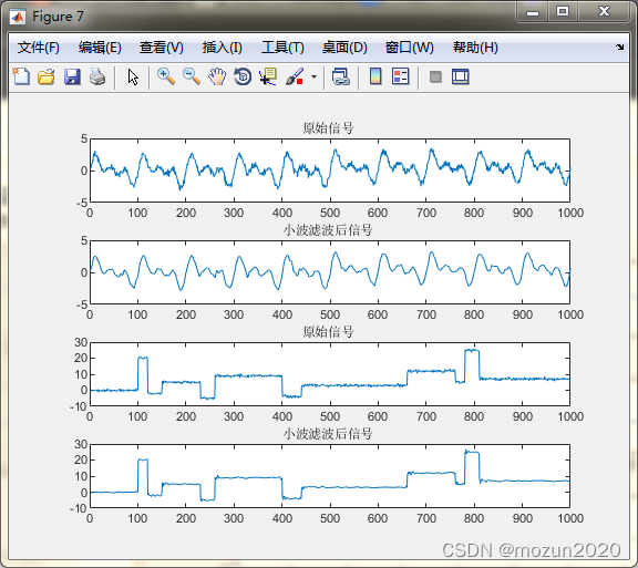
% Mixed signal Mix_Signal_1 Wavelet filtering
figure(7);
subplot(4,1,1);
plot(Mix_Signal_1); %Mix_Signal_1 The original signal
axis([0,1000,-5,5]);
title(' The original signal ');
subplot(4,1,2);
[xd,cxd,lxd] = wden(Mix_Signal_1,'sqtwolog','s','one',2,'db3');
plot(xd); %Mix_Signal_1 Wavelet filtered signal
axis([0,1000,-5,5]);
title(' Wavelet filtered signal ');
% Mixed signal Mix_Signal_2 Wavelet filtering
subplot(4,1,3);
plot(Mix_Signal_2); %Mix_Signal_2 The original signal
axis([0,1000,-10,30]);
title(' The original signal ');
subplot(4,1,4);
[xd,cxd,lxd] = wden(Mix_Signal_2,'sqtwolog','h','sln',3,'db3');
plot(xd); %Mix_Signal_2 Wavelet filtered signal
axis([0,1000,-10,30]);
title(' Wavelet filtered signal ');
Two . Simulation results
3、 ... and . Summary
In the simulation of this section, we mainly deal with the samples with added noise for filtering , The follow-up will depend on the situation , Try to use real noisy samples , For example, filter noisy pictures or noisy speech , Compare the processing effect of each filtering method . Learn one every day MATLAB Little knowledge , Let's learn and make progress together !
版权声明
本文为[mozun2020]所创,转载请带上原文链接,感谢
https://yzsam.com/2022/04/202204231805376679.html
边栏推荐
- Robocode Tutorial 4 - robocode's game physics
- 由tcl脚本生成板子对应的vivado工程
- What are the relationships and differences between threads and processes
- Classes and objects
- QTableWidget使用讲解
- How to ensure the security of futures accounts online?
- 读取excel,int 数字时间转时间
- Svn simple operation command
- Queue solving Joseph problem
- Vulnérabilité d'exécution de la commande de fond du panneau de commande JD - freefuck
猜你喜欢
Docker 安装 Redis
7-21 wrong questions involve knowledge points.
![[UDS unified diagnostic service] IV. typical diagnostic service (6) - input / output control unit (0x2F)](/img/ae/cbfc01fbcc816915b1794a9d70247a.png)
[UDS unified diagnostic service] IV. typical diagnostic service (6) - input / output control unit (0x2F)

cv_ Solution of mismatch between bridge and opencv
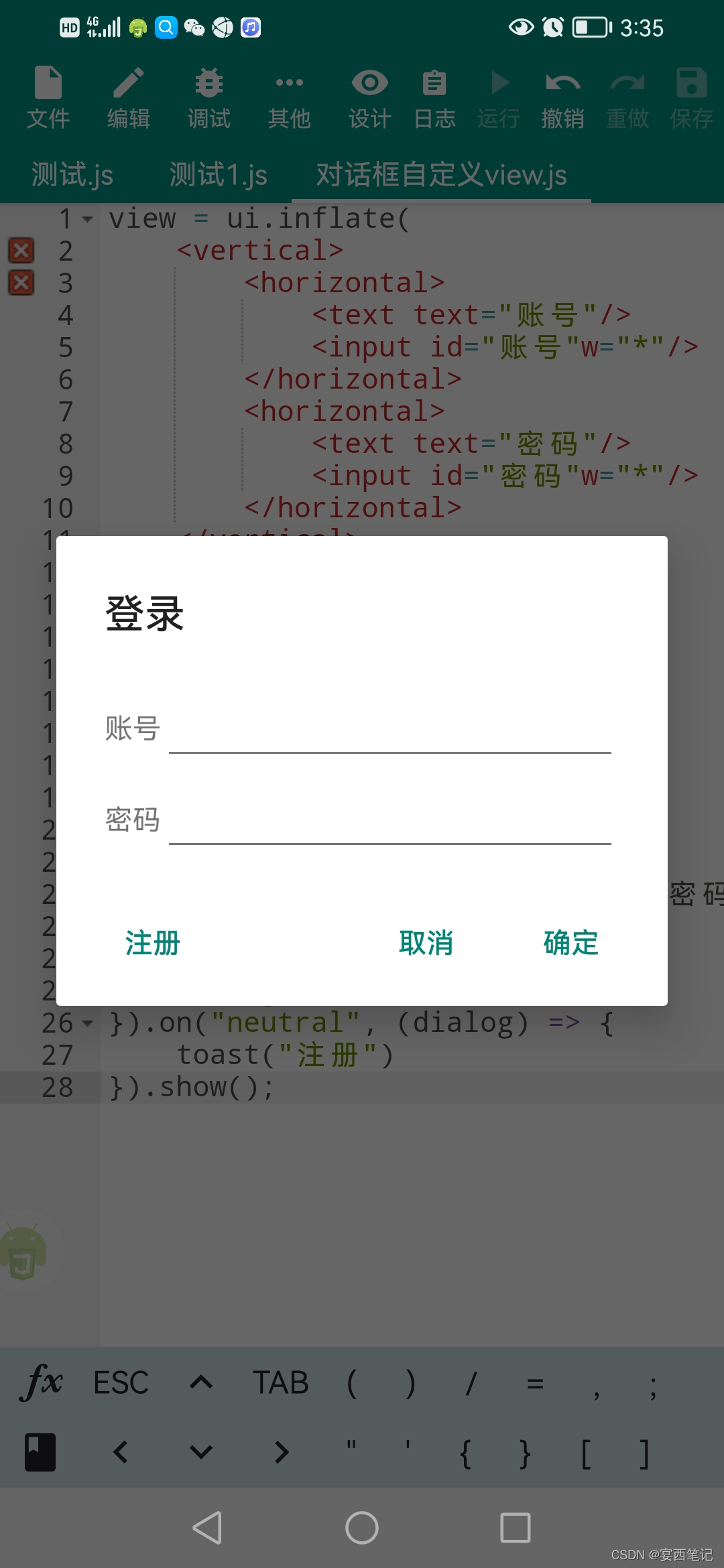
Auto.js 自定义对话框
Scikit learn sklearn 0.18 official document Chinese version
String function in MySQL
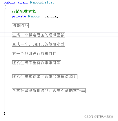
C#的随机数生成
C language loop structure program
深度学习经典网络解析目标检测篇(一):R-CNN

随机推荐
Crawl lottery data
由tcl脚本生成板子对应的vivado工程
[UDS unified diagnostic service] IV. typical diagnostic service (6) - input / output control unit (0x2F)
Visualization of residential house prices
C medium? This form of
Batch export ArcGIS attribute table
Nodejs installation
Docker 安装 MySQL
Rust: a simple example of TCP server and client
SSD硬盘SATA接口和M.2接口区别(详细)总结
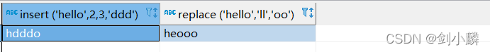
String function in MySQL
Qt读写XML文件(含源码+注释)
Re regular expression
2022 Jiangxi energy storage technology exhibition, China Battery exhibition, power battery exhibition and fuel cell Exhibition
PowerDesigner various font settings; Preview font setting; SQL font settings
.104History
Crawl the product data of Xiaomi Youpin app
软件测试总结
I/O多路复用及其相关详解
QT reading and writing XML files (including source code + comments)