当前位置:网站首页>Logic regression principle and code implementation
Logic regression principle and code implementation
2022-04-23 17:53:00 【Stephen_ Tao】
List of articles
The principle of logical regression
Logistic regression is mainly used to solve binary classification problems , Given an input sample x x x, The output sample belongs to 1 Prediction probability of corresponding category y ^ = P ( y = 1 ∣ x ) \hat{y} = P(y=1|x) y^=P(y=1∣x).
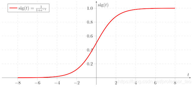
Compared with linear regression , Logistic regression adds a nonlinear function , Such as Sigmoid function , Make the output value in [0,1] In the interval of , And set the threshold for classification .
The main parameters of logistic regression
- Input eigenvector : x ∈ R n x \in R^n x∈Rn( Indicates that the input sample has n n n Eigenvalues ), y ∈ 0 , 1 y \in {0,1} y∈0,1( Label indicating the sample )
- Weight and bias of logistic regression : w ∈ R n w \in R^n w∈Rn, b ∈ R b \in R b∈R
- The predicted results of the output : y ^ = σ ( w T x + b ) = σ ( w 1 x 1 + w 2 x 2 + . . . + w n x n + b ) \hat{y} = \sigma(w^Tx+b)=\sigma(w_1x_1+w_2x_2+...+w_nx_n+b) y^=σ(wTx+b)=σ(w1x1+w2x2+...+wnxn+b)
( σ \sigma σ It's usually Sigmoid function )
The process of logistic regression
- Get your training data ready x ∈ R n × m x \in R^{n \times m} x∈Rn×m( m m m Number of samples , n n n Represents the eigenvalue of each sample ), Training tag data y ∈ R m y \in R^m y∈Rm
- Initialize weights and offsets w ∈ R n w \in R^n w∈Rn, b ∈ R b \in R b∈R
- Data forward propagation y ^ = σ ( w T x + b ) \hat{y} = \sigma(w^Tx+b) y^=σ(wTx+b), The loss is calculated by the maximum likelihood loss function
- The gradient descent method is used to update the weight w w w And offset b b b, Minimum loss function
- The predicted weight and bias are used for data forward propagation , Set classification threshold , Realize the second classification task
Loss function of logistic regression
The square error is used as the loss function in linear regression , In logistic regression, the maximum likelihood loss function is generally used to measure the error between the predicted result and the real value .
The loss value of a single sample is calculated as follows :
L ( y ^ , y ) = − y log y ^ − ( 1 − y ) log ( 1 − y ^ ) L(\hat{y},y)=-y\log\hat{y}-(1-y)\log(1-\hat{y}) L(y^,y)=−ylogy^−(1−y)log(1−y^)
- If the sample belongs to the label 1, be L ( y ^ , y ) = − log y ^ L(\hat{y},y)=-\log\hat{y} L(y^,y)=−logy^, The closer the prediction is to 1, L ( y ^ , y ) L(\hat{y},y) L(y^,y) The smaller the value of
- If the sample belongs to the label 0, be L ( y ^ , y ) = − log ( 1 − y ^ ) L(\hat{y},y)=-\log(1-\hat{y}) L(y^,y)=−log(1−y^), The closer the prediction is to 0, L ( y ^ , y ) L(\hat{y},y) L(y^,y) The smaller the value of
The loss value of all training samples is calculated as follows :
J ( w , b ) = 1 m ∑ i = 1 m L ( y ^ ( i ) , y ( i ) ) J(w,b)=\frac{1}{m}\sum^m_{i=1}L(\hat{y}^{(i)},y^{(i)}) J(w,b)=m1∑i=1mL(y^(i),y(i))
Gradient descent algorithm
The purpose of the gradient descent method is to minimize the loss function , The gradient of the function indicates the direction in which the function changes the fastest .

As shown in the figure above , hypothesis J ( w , b ) J(w,b) J(w,b) It's about w w w and b b b Function of , w , b ∈ R w,b \in R w,b∈R
Calculate the gradient at the initial point , Set the learning rate , Update and iterate the weight and offset parameters , Finally, we can reach the minimum value of the function .
The update formula of weight and offset is :
w = w − α ∂ J ( w , b ) ∂ w w=w-\alpha\frac{\partial{J(w,b)}}{\partial{w}} w=w−α∂w∂J(w,b)
b = b − α ∂ J ( w , b ) ∂ b b=b-\alpha\frac{\partial{J(w,b)}}{\partial{b}} b=b−α∂b∂J(w,b)
notes : among α \alpha α For learning rate , That is, every update w , b w,b w,b Step size of
Gradient calculation based on chain rule
The formula of parameter updating is introduced in the gradient descent method , You can see that the parameter update involves the calculation of the gradient , This section will introduce the flow of gradient calculation in detail .
Simplicity , Make the following assumptions :
- input data x ∈ R 3 × 1 x \in R^{3 \times 1} x∈R3×1(1 Samples ,3 Eigenvalues )
- label y ∈ R y \in R^{} y∈R
- The weight w ∈ R 3 × 1 w \in R^{3 \times1} w∈R3×1
- bias b ∈ R b \in R b∈R
For the sake of understanding , The data flow of logistic regression is represented by flow chart :

1. Calculation J J J About z z z The derivative of
- ∂ J ∂ z = ∂ J ∂ y ^ ∂ y ^ ∂ z \frac{\partial{J}}{\partial{z}}=\frac{\partial{J}}{\partial{\hat{y}}}\frac{\partial{\hat{y}}}{\partial{z}} ∂z∂J=∂y^∂J∂z∂y^
- ∂ J ∂ y ^ = − y y ^ + 1 − y 1 − y ^ \frac{\partial{J}}{\partial{\hat{y}}}=\frac{-y}{\hat{y}}+\frac{1-y}{1-\hat{y}} ∂y^∂J=y^−y+1−y^1−y \quad \quad ∂ y ^ ∂ z = y ^ ( 1 − y ^ ) \frac{\partial{\hat{y}}}{\partial{z}}=\hat{y}(1-\hat{y}) ∂z∂y^=y^(1−y^)
- ∂ J ∂ z = ∂ J ∂ y ^ ∂ y ^ ∂ z = − y ( 1 − y ^ ) + ( 1 − y ) y ^ = y ^ − y \frac{\partial{J}}{\partial{z}}=\frac{\partial{J}}{\partial{\hat{y}}}\frac{\partial{\hat{y}}}{\partial{z}}=-y(1-\hat{y})+(1-y)\hat{y}=\hat{y}-y ∂z∂J=∂y^∂J∂z∂y^=−y(1−y^)+(1−y)y^=y^−y
2. Calculation z z z About w w w and b b b The derivative of
- ∂ z ∂ w 1 = x 1 \frac{\partial{z}}{\partial{w_1}}=x1 ∂w1∂z=x1 \quad \quad ∂ z ∂ w 2 = x 2 \frac{\partial{z}}{\partial{w_2}}=x2 ∂w2∂z=x2 \quad \quad ∂ z ∂ w 3 = x 3 \frac{\partial{z}}{\partial{w_3}}=x3 ∂w3∂z=x3
- ∂ z ∂ b = 1 \frac{\partial{z}}{\partial{b}}=1 ∂b∂z=1
3. Calculation J J J About w w w and b b b The derivative of
- ∂ J ∂ w 1 = ∂ J ∂ z ∂ z ∂ w 1 = ( y ^ − y ) x 1 \frac{\partial{J}}{\partial{w_1}}=\frac{\partial{J}}{\partial{z}}\frac{\partial{z}}{\partial{w_1}}=(\hat{y}-y)x_1 ∂w1∂J=∂z∂J∂w1∂z=(y^−y)x1
- ∂ J ∂ w 2 = ∂ J ∂ z ∂ z ∂ w 2 = ( y ^ − y ) x 2 \frac{\partial{J}}{\partial{w_2}}=\frac{\partial{J}}{\partial{z}}\frac{\partial{z}}{\partial{w_2}}=(\hat{y}-y)x_2 ∂w2∂J=∂z∂J∂w2∂z=(y^−y)x2
- ∂ J ∂ w 3 = ∂ J ∂ z ∂ z ∂ w 3 = ( y ^ − y ) x 3 \frac{\partial{J}}{\partial{w_3}}=\frac{\partial{J}}{\partial{z}}\frac{\partial{z}}{\partial{w_3}}=(\hat{y}-y)x_3 ∂w3∂J=∂z∂J∂w3∂z=(y^−y)x3
- ∂ J ∂ b = ∂ J ∂ z ∂ z ∂ b = ( y ^ − y ) \frac{\partial{J}}{\partial{b}}=\frac{\partial{J}}{\partial{z}}\frac{\partial{z}}{\partial{b}}=(\hat{y}-y) ∂b∂J=∂z∂J∂b∂z=(y^−y)
Vectorization realizes gradient calculation
In the last section , For a single data sample , This paper introduces how to calculate the gradient . But in practice , There can't be only one data sample , Therefore, it is necessary to calculate the gradient based on the loss function of all data samples . In this section, the gradient calculation of multiple data samples will be realized by vectorization , Vectorization is relative to for The way of circulation , Can save a lot of time , Improve the efficiency of operation .
First, declare the structure of the data :
- input data X ∈ R n × m X \in R^{n \times m} X∈Rn×m(m Samples ,n Eigenvalues )
- label Y ∈ R m × 1 Y \in R^{m \times 1} Y∈Rm×1
- The weight W ∈ R n × 1 W \in R^{n \times1} W∈Rn×1
- bias b ∈ R b \in R b∈R
The gradient descent process is as follows :
- Z = W T X + b Z=W^TX+b Z=WTX+b \quad Z ∈ R 1 × m Z\in R^{1\times m} Z∈R1×m
- Y ^ = σ ( Z ) \hat{Y}=\sigma(Z) Y^=σ(Z) \quad Y ^ ∈ R 1 × m \hat{Y}\in R^{1\times m} Y^∈R1×m
- ∂ J ∂ z = Y ^ − Y \frac{\partial{J}}{\partial{z}}=\hat{Y}-Y ∂z∂J=Y^−Y \quad ∂ J ∂ z ∈ R 1 × m \frac{\partial{J}}{\partial{z}}\in R^{1\times m} ∂z∂J∈R1×m
- ∂ J ∂ W = 1 m X ( Y ^ − Y ) T \frac{\partial{J}}{\partial{W}}=\frac{1}{m}X(\hat{Y}-Y)^T ∂W∂J=m1X(Y^−Y)T \quad ∂ J ∂ W ∈ R n × 1 \frac{\partial{J}}{\partial{W}}\in R^{n\times 1} ∂W∂J∈Rn×1
- ∂ J ∂ b = 1 m n p . s u m ( Y ^ − Y ) \frac{\partial{J}}{\partial{b}}=\frac{1}{m}np.sum(\hat{Y}-Y) ∂b∂J=m1np.sum(Y^−Y) \quad ∂ J ∂ b ∈ R \frac{\partial{J}}{\partial{b}}\in R ∂b∂J∈R
- W = W − α ∂ J ∂ W W = W-\alpha \frac{\partial{J}}{\partial{W}} W=W−α∂W∂J \quad b = b − α ∂ J ∂ b b= b-\alpha \frac{\partial{J}}{\partial{b}} b=b−α∂b∂J
Logistic regression code implementation
Obtain secondary classification data
from sklearn.datasets import load_iris,make_classification
from sklearn.model_selection import train_test_split
import tensorflow as tf
import numpy as np

#  Generate 500 A sample points , The sample category is only 2 Kind of , The eigenvalues of each sample are 4 individual
X,Y=make_classification(n_samples=500,n_features=4,n_classes=2)

#  take 30% As a test set ,70% Data as a training set
x_train,x_test,y_train,y_test = train_test_split(X,Y,test_size=0.3)
print("X:",X.shape)
print("Y:",Y.shape)
print("x_train:",x_train.shape)
print("x_test:",x_test.shape)
print("y_train:",y_train.shape)
print("y_test:",y_test.shape)
The output is :
X: (500, 4)
Y: (500,)
x_train: (350, 4)
x_test: (150, 4)
y_train: (350,)
y_test: (150,)
Define initialization module
def initialize_with_zeros(shape):
    """  Create a shape as  (shape, 1)  Of w Parameters and b=0. return:w, b """
    w = np.zeros((shape, 1))
    b = 0
    return w, b
Define loss function and gradient
def basic_sigmoid(x):
    """  Calculation sigmoid function  """
    s = 1 / (1 + np.exp(-x))
    return s

def propagate(w, b, X, Y):
    """  Parameters :w,b,X,Y: Network parameters and data  Return:  Loss cost、 Parameters W Gradient of dw、 Parameters b Gradient of db """
    m = X.shape[1]

    # w (n,1), x (n, m)
    A = basic_sigmoid(np.dot(w.T, X) + b)
    #  Calculate the loss
    cost = -1 / m * np.sum(Y * np.log(A) + (1 - Y) * np.log(1 - A))
    dz = A - Y
    dw = 1 / m * np.dot(X, dz.T)
    db = 1 / m * np.sum(dz)

    cost = np.squeeze(cost)

    grads = {
    "dw": dw,
             "db": db}
    return grads, cost
Define gradient descent algorithm
def optimize(w, b, X, Y, num_iterations, learning_rate):
    """  Parameters : w: The weight ,b: bias ,X features ,Y The target ,num_iterations The total number of iterations ,learning_rate Learning rate  Returns: params: Updated parameter Dictionary  grads: gradient  costs: Loss results  """

    costs = []

    for i in range(num_iterations):

        #  Gradient update calculation function
        grads, cost = propagate(w, b, X, Y)

        #  Take out the gradient of two partial parameters
        dw = grads['dw']
        db = grads['db']

        #  Calculate according to the gradient descent formula
        w = w - learning_rate * dw
        b = b - learning_rate * db

        if i % 100 == 0:
            costs.append(cost)
            print(" Loss results  %i: %f" %(i, cost))


    params = {
    "w": w,"b": b}

    grads = {
    "dw": dw,"db": db}
    return params, grads, costs
Define prediction module
def predict(w, b, X):
    '''  Use the trained parameters to predict  return: Predicted results  '''

    m = X.shape[1]
    y_prediction = np.zeros((1, m))
    w = w.reshape(X.shape[0], 1)

    #  The result of the calculation is
    A = basic_sigmoid(np.dot(w.T, X) + b)

    for i in range(A.shape[1]):

        if A[0, i] <= 0.5:
            y_prediction[0, i] = 0
        else:
            y_prediction[0, i] = 1

    return y_prediction
Define a logistic regression model
def model(x_train, y_train, x_test, y_test, num_iterations=2000, learning_rate=0.0001):
    """ """

    #  Modify the data shape
    x_train = x_train.reshape(-1, x_train.shape[0])
    x_test = x_test.reshape(-1, x_test.shape[0])
    y_train = y_train.reshape(1, y_train.shape[0])
    y_test = y_test.reshape(1, y_test.shape[0])
    print(x_train.shape)
    print(x_test.shape)
    print(y_train.shape)
    print(y_test.shape)

    # 1、 Initialize parameters
    w, b = initialize_with_zeros(x_train.shape[0])

    # 2、 gradient descent
    # params: Updated network parameters
    # grads: Last gradient
    # costs: Loss list updated each time
    params, grads, costs = optimize(w, b, x_train, y_train, num_iterations, learning_rate)

    #  Get training parameters
    #  Predicted results
    w = params['w']
    b = params['b']
    y_prediction_train = predict(w, b, x_train)
    y_prediction_test = predict(w, b, x_test)

    #  Print accuracy
    print(" Training set accuracy : {} ".format(100 - np.mean(np.abs(y_prediction_train - y_train)) * 100))
    print(" Test set accuracy : {} ".format(100 - np.mean(np.abs(y_prediction_test - y_test)) * 100))

    return None
Run the model
model(x_train, y_train, x_test, y_test, num_iterations=3000, learning_rate=0.01)
Set the number of iterations to 3000, The learning rate is set to 0.01, Running will get the following results :
(4, 350)
(4, 150)
(1, 350)
(1, 150)
 Loss results  0: 0.693147
 Loss results  100: 0.685711
 Loss results  200: 0.681650
 Loss results  300: 0.679411
 Loss results  400: 0.678165
 Loss results  500: 0.677465
 Loss results  600: 0.677069
 Loss results  700: 0.676843
 Loss results  800: 0.676713
 Loss results  900: 0.676639
 Loss results  1000: 0.676595
 Loss results  1100: 0.676570
 Loss results  1200: 0.676556
 Loss results  1300: 0.676547
 Loss results  1400: 0.676542
 Loss results  1500: 0.676539
 Loss results  1600: 0.676538
 Loss results  1700: 0.676537
 Loss results  1800: 0.676536
 Loss results  1900: 0.676536
 Loss results  2000: 0.676535
 Loss results  2100: 0.676535
 Loss results  2200: 0.676535
 Loss results  2300: 0.676535
 Loss results  2400: 0.676535
 Loss results  2500: 0.676535
 Loss results  2600: 0.676535
 Loss results  2700: 0.676535
 Loss results  2800: 0.676535
 Loss results  2900: 0.676535
 Training set accuracy : 60.57142857142857
 Test set accuracy : 56.0
The change of loss function value is shown in the figure below :

summary
This paper introduces the principle of logistic regression in detail , And make use of Python A case of realizing logical regression . From the running results, we can see that , As the number of iterations increases , The value of the loss function does not always drop close to 0 The location of , It's stable 0.6 near . meanwhile , The prediction accuracy of the training set is 60.57%, The accuracy of the prediction for the test set is 56%. Therefore, although logical regression is simple and easy to understand , The interpretability of the model is very good , But because the form of the model is relatively simple , Can't fit the real distribution of data well , So the accuracy is often not very high .
版权声明
本文为[Stephen_ Tao]所创,转载请带上原文链接,感谢
https://yzsam.com/2022/04/202204230548468772.html
边栏推荐
- .104History
- Click Cancel to return to the previous page and modify the parameter value of the previous page, let pages = getcurrentpages() let prevpage = pages [pages. Length - 2] / / the data of the previous pag
- 2022江西储能技术展会,中国电池展,动力电池展,燃料电池展
- Listen for click events other than an element
- Utilisation de la liste - Ajouter, supprimer et modifier la requête
- JS interview question: FN call. call. call. Call (FN2) parsing
- Examination question bank and online simulation examination of the third batch (main person in charge) of special operation certificate of safety officer a certificate in Guangdong Province in 2022
- 2022 judgment questions and answers for operation of refrigeration and air conditioning equipment
- 2021长城杯WP
- 48. 旋转图像
猜你喜欢
Comparison between xtask and kotlin coroutine

2022年上海市安全员C证操作证考试题库及模拟考试

102. 二叉树的层序遍历
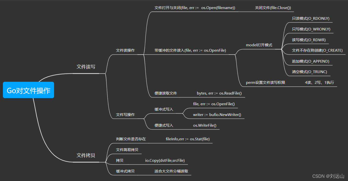
Go对文件操作

Halo open source project learning (II): entity classes and data tables

958. 二叉树的完全性检验

2022 Jiangxi Photovoltaic Exhibition, China distributed Photovoltaic Exhibition, Nanchang solar energy utilization Exhibition

开源按键组件Multi_Button的使用,含测试工程
Open source key component multi_ Button use, including test engineering

JS get link? The following parameter name or value, according to the URL? Judge the parameters after
随机推荐
Element calculation distance and event object
This point in JS
Uniapp custom search box adaptation applet alignment capsule
2022 Shanghai safety officer C certificate operation certificate examination question bank and simulation examination
JS high frequency interview questions
Welcome to the markdown editor
Gaode map search, drag and drop query address
2022江西储能技术展会,中国电池展,动力电池展,燃料电池展
239. Maximum value of sliding window (difficult) - one-way queue, large top heap - byte skipping high frequency problem
Operation of 2022 mobile crane driver national question bank simulation examination platform
122. 买卖股票的最佳时机 II-一次遍历
Ring back to origin problem - byte jumping high frequency problem
2021长城杯WP
Special effects case collection: mouse planet small tail
Go的Gin框架学习
Hcip fifth experiment
2022 tea artist (primary) examination simulated 100 questions and simulated examination
油猴网站地址
关于gcc输出typeid完整名的方法
2022年茶艺师(初级)考试模拟100题及模拟考试