一、 设计目标

学习常见的SLAM知识，使用Cartographer算法实现二维栅格化地图的建立，并进行优化和测试。

二、 技术要求

查找建图相关资料，了解常用的激光SLAM算法；
安装Linux系统，建议Ubuntu18.04；
安装ROS环境并学习其基本操作；
完成谷歌Cartographer算法建图环境搭建；
使用Cartagrapher算法进行建图测试；
学习算法原理，对算法进行优化及测试。

三、 设计方案

1. 激光SLAM简介

SLAM (simultaneous localization and mapping) , 即时定位与地图构建，或称并发建图与定位。问题可以描述为：将一个机器人放入未知环境中的未知位置，是否有办法让机器人一边移动一边逐步描绘出此环境完全的地图，所谓完全的地图（a consistent map）是指不受障碍行进到房间可进入的每个角落。近年来，智能机器人技术在世界范围内得到快速发展。从室内、外搬运机器人，到自动驾驶汽车，再到空中无人机、水下探测机器人等，智能机器人的运用都得到了巨大突破。
激光雷达已经被证明在低照度、少纹理等环境中更加有效，可以提供高信噪比的观测数据，精度高，测量距离远，可以准确获得目标的三维信息。激光SLAM技术相对成熟，在工业 AGV、无人驾驶领域已经得到广泛应用。
激光SLAM利用二维激光测距仪或者三维激光测距仪对场景进行感知，利用返回的点云数据估计车辆的运动，并输出场景建模的结果。激光SLAM的工作原理也可以分为前端和后端2个部分，前端用于获取扫描数据，通过帧间点云的匹配估计车辆的运动关系，后端用于进行优化计算，闭环检测以及场景建模的输出等。在前端计算中，常用的点云匹配方法有迭代最近邻（Iterative Closest Point, ICP）算法及其变种算法，如PI-IC，相关性扫描匹配方法 (Correlation Scan Match, CSM)，特征匹配法[8]和梯度优化方法等，在后端优化方法中，常用的方法有基于滤波器的方法和基于图优化的方法等。目前常见 的 二 维 激 光SLAM方 法 有：Gmapping-SLAM， Hector-SLAM，Karto SLAM和 Cartographer等，三 维 激 光SLAM方 法有LOAM，LeGO-LOAM和 MC2SLAM等。本次我们主要以谷歌开源的Cartographer建图算法进行相关的算法测试与改进。

2. Cartographer简介与使用

1) Cartographer简介

2016年10月5日，谷歌宣布开放一个名为cartographer的即时定位与地图建模库，开发人员可以使用该库实现机器人在二维或三维条件下的定位及建图功能。cartograhper的设计目的是在计算资源有限的情况下，实时获取相对较高精度的2D地图。考虑到基于模拟策略的粒子滤波方法在较大环境下对内存和计算资源的需求较高，cartographer采用基于图网络的优化方法。目前cartographer主要基于激光雷达来实现SLAM，谷歌希望通过后续的开发及社区的贡献支持更多的传感器和机器人平台，同时不断增加新的功能。
首先是对整个功能包的安装过程cartographer功能包已经与ROS集成，现在已经提供二进制安装包，本次采用源码编译的方式进行安装。为了不与已有功能包冲突，最好为cartographer专门创建一个工作空间，这里我们新创建了一个工作空间google_ws，然后使用如下步骤下载源码并完成编译。

• 安装工具 可以使用如下命令安装工具：

$ sudo apt-get update
$ sudo apt-get install -y python-wstool python-rosdep ninja-build

• 初始化工作空间 使用如下命令初始化工作空间：

$ cd google_ws
$ wstool init src

• 加入cartographer_ros.rosinstall并更新依赖 命令如下：

$ wstool merge -t src https://raw.githubusercontent.com/googlecartographer/cartographer_ros/master/cartographer_ros.rosinstall
$ wstool update -t src

• 安装依赖并下载cartographer相关功能包 命令如下：

$ rosdep update
$ rosdep install --from-paths src --ignore-src --rosdistro=${ROS_DISTRO} -y

• 编译并安装 命令如下

$ catkin_make_isolated --install --use-ninja
$ source install_isolated/setup.bash

如果下载服务器无法连接，也可以使用如下命令修改ceres-solver源码的下载地址为

https://github.com/ceres-solver/ceres-solver.git

$ gedit google_ws/src/.rosinstall

改完成后重新运行编译安装的命令，如果没有出错，则cartographer的相关功能包安装成功。

2) 官方demo的演示

首先，下载官方提供的2D Cartographer功能包，复现并测试功能包的运行情况。

$ wget -P ~/Downloads https://storage.googleapis.com/cartographer-public-data/bags/backpack_2d/cartographer_paper_deutsches_museum.bag

接着，运行Cartographer的demo文件，复现该文件的建图功能。如下图3-1、3-2所示：

$ roslaunch cartographer_ros demo_backpack_2d.launch bag_filename:=${
    HOME}/Downloads/cartographer_paper_deutsches_museum.bag

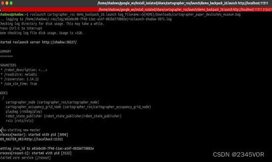
图3-1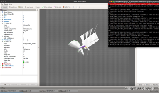

图3-2
另起终端，输入下列指令，如图3-3查看该建图功能中订阅的话题：

$ rostopic list

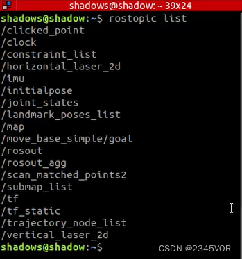
图3-3
另起一个终端，查看该工程的tf配置，如下图3-4所示：

$ rosrun rqt_tf_tree rqt_tf_tree

图3-5
另起终端，输入下列指令，查看该建图功能运行的相关节点，如图3-5所示：

$ rosrun rqt_graph rqt_graph

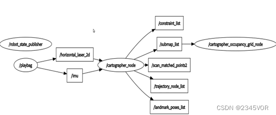
图3-5

3. 阿克曼模型测试

通过对官方功能包的功能复现，我们可以更好的学习到Cartographer与传统2D建图算法相比的优缺点与异同。所以我们将五个关键任务中第一部分在ros中搭建的阿克曼运动模型应用起来，通过配置其相关参数，使他可以使用Cartographer在仿真环境下进行相关的建图与导航功能的测试，加深对第一部分阿克曼运动的理解，同时也强化Cartographer在阿克曼运动中的实际建图效果。

1) SLAM建图

首先，需要对谷歌Cartographer建图功能包中相关的数据进行一些配置，由于普通用的基本为2D或者3D激光雷达，如我的机器人使用2D激光，这里按照这个进行简介，我们移植到自己机器人需做三件事：
第一件：一定要把Cartography和自己ROS 工作空间隔离开，不然存在问题，两个不是用相同编译器进行。
第二件：更改demo_revo_lds.launch使其匹配自己的机器人
第三件：根据自己机器人配置的TF结构对cartography的配置文件进行更改，这里主要会更改lua脚本，这里使用revo_lds.lua。
更改demo_revo_lds.launch，这里主要删除不需要配置，如跑bag的节点和更改我们自己发布的2D激光雷达的数据，更改后的如下：

<launch>
  <param name="/use_sim_time" value="false" />

  <node name="cartographer_node" pkg="cartographer_ros" type="cartographer_node" args=" -configuration_directory $(find cartographer_ros)/configuration_files -configuration_basename revo_lds.lua" output="screen">
    <remap from="scan" to="scan" />
  </node>
  <node name="cartographer_occupancy_grid_node" pkg="cartographer_ros" type="cartographer_occupancy_grid_node" args="-resolution 0.05" />

  <node name="rviz" pkg="rviz" type="rviz" required="true" args="-d $(find cartographer_ros)/configuration_files/demo_2d.rviz" />
</launch>

更改revo_lds.lua主要也是对我们没用到的配置进行删除处理，这里主要看我们发布的坐标系更改后如下：

include "map_builder.lua"
include "trajectory_builder.lua"

options = {
    
  map_builder = MAP_BUILDER,
  trajectory_builder = TRAJECTORY_BUILDER,
  map_frame = "map",
  tracking_frame = "laser_link",
  published_frame = "laser_link",
  odom_frame = "odom",
  provide_odom_frame = true,
  publish_frame_projected_to_2d = false,
  use_pose_extrapolator = true,
  use_odometry = false,
  use_nav_sat = false,
  use_landmarks = false,
  num_laser_scans = 1,
  num_multi_echo_laser_scans = 0,
  num_subdivisions_per_laser_scan = 1,
  num_point_clouds = 0,
  lookup_transform_timeout_sec = 0.2,
  submap_publish_period_sec = 0.3,
  pose_publish_period_sec = 5e-3,
  trajectory_publish_period_sec = 30e-3,
  rangefinder_sampling_ratio = 1.,
  odometry_sampling_ratio = 1.,
  fixed_frame_pose_sampling_ratio = 1.,
  imu_sampling_ratio = 1.,
  landmarks_sampling_ratio = 1.,
}

MAP_BUILDER.use_trajectory_builder_2d = true

TRAJECTORY_BUILDER_2D.submaps.num_range_data = 35
TRAJECTORY_BUILDER_2D.min_range = 0.3
TRAJECTORY_BUILDER_2D.max_range = 8.
TRAJECTORY_BUILDER_2D.missing_data_ray_length = 1.
TRAJECTORY_BUILDER_2D.use_imu_data = false
TRAJECTORY_BUILDER_2D.use_online_correlative_scan_matching = true
TRAJECTORY_BUILDER_2D.real_time_correlative_scan_matcher.linear_search_window = 0.1
TRAJECTORY_BUILDER_2D.real_time_correlative_scan_matcher.translation_delta_cost_weight = 10.
TRAJECTORY_BUILDER_2D.real_time_correlative_scan_matcher.rotation_delta_cost_weight = 1e-1

POSE_GRAPH.optimization_problem.huber_scale = 1e2
POSE_GRAPH.optimize_every_n_nodes = 35
POSE_GRAPH.constraint_builder.min_score = 0.65
return options

有些比较明了的参数根据自己的要求进行更改，其他的我们暂时默认就好。 配置完成后回到google_ws路径下，使用如下命令再次编译：

$ catkin_make_isolated --install --use-ninja

打开仿真环境下的gazebo可视化界面，加载雷达和相关的传感器数据，如下图3-6所示：

$ roslaunch bringup ares_gazebo_rviz.launch

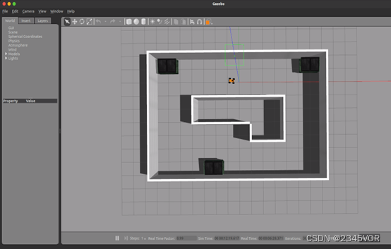
图3-6
启动键盘控制：

$ rosrun ares_description keyboard_teleop.py

运行cartographer的建图功能，操纵键盘开始建图，如图3-7、3-8、3-9所示：

$ roslaunch cartographer_ros demo_revo_lds.launch

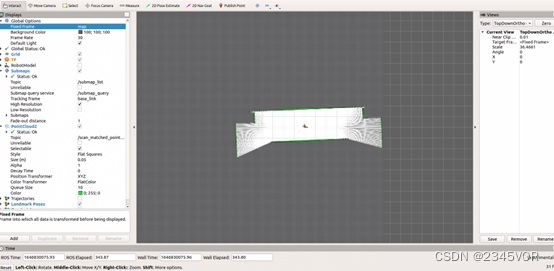
图3-7

图3-8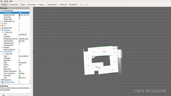

图3-9
建图完成后，运行下列程序，执行保存地图的功能，为后续的导航提供所需地图，如图3-10所示：

$ rosrun map_server map_saver -f ~/map

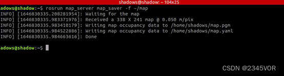
图3-10
2) SLAM导航
上述的建图完成后，我们测试一下阿克曼模型的导航功能，考虑到阿克曼模型和真车类似，base_local_planner 和dwa_local_planner不适应阿克曼，所以建图的过程我们选用teb算法进行仿真，打开仿真环境下的gazebo可视化界面，如图3-11，加载雷达和相关的传感器数据：

$ roslaunch bringup ares_gazebo_rviz.launch

图3-11
首先我们查看导航功能的move_base.launch文件的相关配置：

<launch>

   <node pkg="move_base" type="move_base" respawn="false" name="move_base" output="screen">
    <rosparam file="$(find bringup)/param/costmap_common_params.yaml" command="load" ns="global_costmap" /> 
    <rosparam file="$(find bringup)/param/costmap_common_params.yaml" command="load" ns="local_costmap" />
    <rosparam file="$(find bringup)/param/local_costmap_params.yaml" command="load" />
    <rosparam file="$(find bringup)/param/global_costmap_params.yaml" command="load" /> 
    <rosparam file="$(find bringup)/param/teb_local_planner_params.yaml" command="load" />
    <rosparam file="$(find bringup)/param/move_base_params.yaml" command="load" />
    
    <param name="base_local_planner" value="teb_local_planner/TebLocalPlannerROS" />
    <!--<param name="controller_frequency" value="10" /> <param name="controller_patiente" value="15.0"/>-->
   </node>


   	<node name="map_server" pkg="map_server" type="map_server" args="$(find bringup)/map/map.yaml" output="screen">
                <param name="frame_id" value="map"/>
    </node>

    <!--<node pkg="tf" type="static_transform_publisher" name="odom_to_map" args="0 0 0 0 0 0 1 /odom /map 100" />-->

    <!--<include file="$(find bringup)/launch/robot_amcl.launch.xml" />-->

   <node name="nav_sim" pkg="ares_description" type="nav_sim.py" >
    </node>

   <arg name="use_map_topic" default="True"/>
    <arg name="scan_topic" default="/scan"/> 
    <arg name="initial_pose_x" default="-0.5"/>
    <arg name="initial_pose_y" default="0.0"/>
    <arg name="initial_pose_a" default="0.0"/>
    <arg name="odom_frame_id" default="odom"/>
    <arg name="base_frame_id" default="base_footprint"/>
    <arg name="global_frame_id" default="map"/>
  <node pkg="amcl" type="amcl" name="amcl">
      <param name="use_map_topic" value="$(arg use_map_topic)"/>
      <!-- Publish scans from best pose at a max of 10 Hz -->
      <param name="odom_model_type" value="diff"/>
      <param name="odom_alpha5" value="0.1"/>
      <param name="gui_publish_rate" value="10.0"/>
      <param name="laser_max_beams" value="810"/>
      <param name="laser_max_range" value="-1"/>
      <param name="min_particles" value="500"/>
      <param name="max_particles" value="5000"/>
      <param name="kld_err" value="0.05"/>
      <param name="kld_z" value="0.99"/>
      <param name="odom_alpha1" value="0.2"/>
      <param name="odom_alpha2" value="0.2"/>
      <!-- translation std dev, m -->
      <param name="odom_alpha3" value="0.2"/>
      <param name="odom_alpha4" value="0.2"/>
      <param name="laser_z_hit" value="0.5"/>
      <param name="laser_z_short" value="0.05"/>
      <param name="laser_z_max" value="0.05"/>
      <param name="laser_z_rand" value="0.5"/>
      <param name="laser_sigma_hit" value="0.2"/>
      <param name="laser_lambda_short" value="0.1"/>
      <param name="laser_model_type" value="likelihood_field"/>
      <!-- <param name="laser_model_type" value="beam"/> -->
      <param name="laser_likelihood_max_dist" value="2.0"/>
      <param name="update_min_d" value="0.1"/>
      <param name="update_min_a" value="0.2"/>
      <param name="odom_frame_id" value="$(arg odom_frame_id)"/> 
      <param name="base_frame_id" value="$(arg base_frame_id)"/> 
      <param name="global_frame_id" value="$(arg global_frame_id)"/>
      <param name="resample_interval" value="1"/>
      <!-- Increase tolerance because the computer can get quite busy -->
      <param name="transform_tolerance" value="1.0"/>
      <param name="recovery_alpha_slow" value="0.0"/>
      <param name="recovery_alpha_fast" value="0.0"/>
      <param name="initial_pose_x" value="$(arg initial_pose_x)"/>
      <param name="initial_pose_y" value="$(arg initial_pose_y)"/>
      <param name="initial_pose_a" value="$(arg initial_pose_a)"/>
      <remap from="/scan" to="$(arg scan_topic)"/>
      <remap from="/tf_static" to="/tf_static"/>
    </node>

   </launch>

该部分加载了导航必要的全局与局部规划的相关配置参数以及代价地图的相关配置参数，并且考虑到没有GPS为小车做定位，选用amcl对阿克曼小车进行更加精准的定位。
重启一个终端，运行下列命令，如图3-12：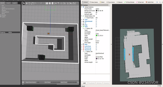

$ roslaunch bringup move_base.launch

图3-12
使用rviz中的2D Nav Goal发布目标点，Ares阿克曼小车就会自动导航到该点，效果如下图3-13、3-14、3-15所示：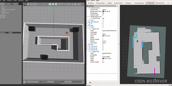

图3-13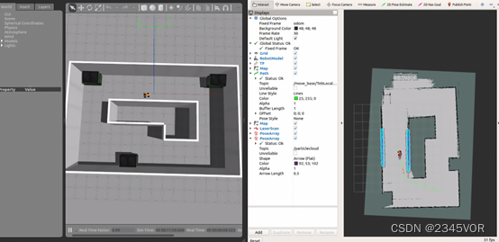

图3-14

图3-15

四、 总结与展望

至此，cartographer的官方功能包的复现和对自己的阿克曼模型的建图验证，可以证明该建图算法的建图效果要优于gmapping等传统的2D建图效果，主要体现在cartographer的回环检测功能，在建图过程中我们可以发现，该算法可以不断地对时所建的地图进行不断地调整和优化，这是传统普通的slam算法所没有的功能；后续的时间中我们将考虑融合搭建在阿克曼车上的rgbd相机，实现相机+激光雷达融合的rtabmap slam算法，并不断优化cartographer功能包的相关参数以及阿克曼的相关配置。在导航方面，将加入第四部分中优化后的A*算法来进行相关的导航功能。以及控制阿克曼智能车实现导航过程中的物体目标识别和车道线检测与巡线的功能，并实现与上位机的实时通讯。