当前位置:网站首页>1.1-Regression
1.1-Regression
2022-08-11 07:51:00 【A boa constrictor. 6666】
文章目录
一、模型model
一个函数function的集合:
- 其中wi代表权重weight,b代表偏置值bias
- 𝑥𝑖Different properties can be taken,如: 𝑥𝑐𝑝, 𝑥ℎ𝑝, 𝑥𝑤,𝑥ℎ…
𝑦 = 𝑏 + ∑ w i x i 𝑦=𝑏+∑w_ix_i y=b+∑wixi
我们将𝑥𝑐𝑝Take it out as an unknown quantity,to find an optimal linear modelLinear model:
y = b + w ∙ X c p y = b + w ∙Xcp~ y=b+w∙Xcp
二、better functionfunction
损失函数Loss function 𝐿:
L的输入Input是一个函数 f ,输出outputis a specific value,And this value is the function used to evaluate the input f 到底有多坏
y ^ n \widehat{y}^n yn代表真实值,而 f ( x c p n ) f(x^n_{cp}) f(xcpn)代表预测值, L ( f ) L(f) L(f)represents the total error between the true value and the predicted value
L ( f ) = ∑ n = 1 10 ( y ^ n − f ( x c p n ) ) 2 L(f)=\sum_{n=1}^{10}(\widehat{y}^n-f(x^n_{cp}))^2 L(f)=n=1∑10(yn−f(xcpn))2将函数 f 用w,b替换,则可以写成下面这样
L ( w , b ) = ∑ n = 1 10 ( y ^ n − ( b + w ⋅ x c p n ) ) 2 L(w,b)=\sum_{n=1}^{10}(\widehat{y}^n-(b+w \cdot x^n_{cp}))^2 L(w,b)=n=1∑10(yn−(b+w⋅xcpn))2当 L 越小时,则说明该函数 f 越好,That is, the model is better.Each point in the graph below represents a function f

三、best functionfunction
梯度下降Gradient Descent:It is the process of finding the best function
$f^{ } represents the best function f u n c t i o n , represents the best functionfunction, represents the best functionfunction,w{*},b{ }:$represents the best weightweight和偏置值bias
f ∗ = a r g m i n f L ( f ) f^{*} =arg \underset{f}{min} L(f) f∗=argfminL(f)
w ∗ , b ∗ = a r g m i n w , b L ( w , b ) w^{*},b^{*}=arg \underset{w,b}{min} L(w,b) w∗,b∗=argw,bminL(w,b)
= a r g m i n w , b ∑ n = 1 10 ( y ^ n − ( b + w ⋅ x c p n ) ) 2 =arg \underset{w,b}{min}\sum_{n=1}^{10}(\widehat{y}^n-(b+w \cdot x^n_{cp}))^2 =argw,bmin∑n=110(yn−(b+w⋅xcpn))2
3.1 一维函数
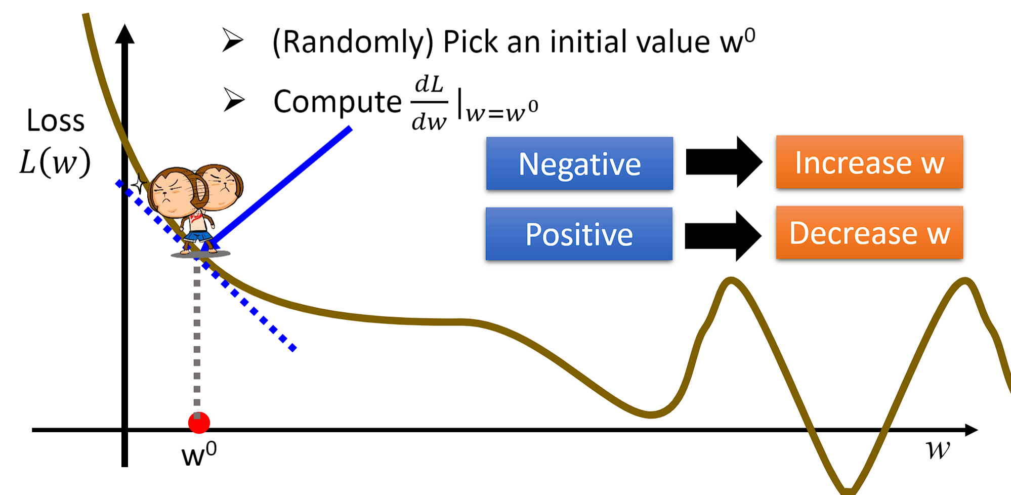
下图代表Lossfunction for gradient descent(Gradient Descent)的过程,首先随机选择一个 w 0 w^{0} w0.at that pointw求微分,如果为负数,Then we increase w 0 w^{0} w0的值;如果为正数,Then we reduce w 0 w^{0} w0的值.
- w ∗ = a r g m i n w L ( w ) w^{*}=arg\underset{w}{min}L(w) w∗=argwminL(w)
- w 0 = − η d L d w ∣ w w^{0}=-\eta\frac{dL}{dw}|_{w} w0=−ηdwdL∣w,其中 η 代表学习率:Learning rate,means the step size for each move(step)
- w 1 ← w 0 − η d L d w ∣ w = w 0 w^{1}\leftarrow w^{0}-\eta\frac{dL}{dw}|_{w=w^{0}} w1←w0−ηdwdL∣w=w0, w 1 w1 w1represents the initial point w 0 w^{0} w0The next point to move,Iterate like this(Iteration)下去,Eventually our local optimum will be found:Local optimal solution


3.2 二维函数
- for two-dimensional functions$Loss $ L ( w , b ) L(w,b) L(w,b)Find gradient descent: [ ∂ L ∂ w ∂ L ∂ b ] g r a d i e n t \begin{bmatrix} \frac{\partial L}{\partial w}\\ \frac{\partial L}{\partial b} \end{bmatrix}_{gradient} [∂w∂L∂b∂L]gradient
- w ∗ , b ∗ = a r g m i n w , b L ( w , b ) w^{*},b^{*}=arg \underset{w,b}{min} L(w,b) w∗,b∗=argw,bminL(w,b)
- 随机初始化 w 0 , b 0 w^{0},b^{0} w0,b0,然后计算 ∂ L ∂ w ∣ w = w 0 , b = b 0 \frac{\partial L}{\partial w}|_{w=w^{0},b=b^{0}} ∂w∂L∣w=w0,b=b0和 ∂ L ∂ b ∣ w = w 0 , b = b 0 \frac{\partial L}{\partial b}|_{w=w^{0},b=b^{0}} ∂b∂L∣w=w0,b=b0:
- w 1 ← w 0 − η ∂ L ∂ w ∣ w = w 0 , b = b 0 w^{1}\leftarrow w^{0}-\eta\frac{\partial L}{\partial w}|_{w=w^{0},b=b^{0}} w1←w0−η∂w∂L∣w=w0,b=b0
- b 1 ← b 0 − η ∂ L ∂ b ∣ w = w 0 , b = b 0 b^{1}\leftarrow b^{0}-\eta\frac{\partial L}{\partial b}|_{w=w^{0},b=b^{0}} b1←b0−η∂b∂L∣w=w0,b=b0

3.3 局部最优解和全局最优解
公式化(Formulation) ∂ L ∂ w \frac{\partial L}{\partial w} ∂w∂L和$
\frac{\partial L}{\partial b}$:- L ( w , b ) = ∑ n = 1 10 ( y ^ n − ( b + w ⋅ x c p n ) ) 2 L(w,b)=\sum_{n=1}^{10}(\widehat{y}^n-(b+w \cdot x^n_{cp}))^2 L(w,b)=∑n=110(yn−(b+w⋅xcpn))2
- ∂ L ∂ w = 2 ∑ n = 1 10 ( y ^ n − ( b + w ⋅ x c p n ) ) ( − x c p n ) \frac{\partial L}{\partial w}=2\sum_{n=1}^{10}(\widehat{y}^n-(b+w \cdot x^n_{cp}))(-x^{n}_{cp}) ∂w∂L=2∑n=110(yn−(b+w⋅xcpn))(−xcpn)
- ∂ L ∂ b = 2 ∑ n = 1 10 ( y ^ n − ( b + w ⋅ x c p n ) ) \frac{\partial L}{\partial b}=2\sum_{n=1}^{10}(\widehat{y}^n-(b+w \cdot x^n_{cp})) ∂b∂L=2∑n=110(yn−(b+w⋅xcpn))
在非线性系统中,There may be multiple local optimal solutions:

3.4 模型的泛化(Generalization)能力
将根据lossThe best model found by the function is taken out,Calculate it separately on the training set(Training Data)和测试集(Testing Data)mean squared error on (Average Error),Of course, we only care about how well the model performs on the test set.
- y = b + w ∙ x c p y = b + w ∙x_{cp} y=b+w∙xcp Average Error=35.0
Because the mean square error of the original model is still relatively large,为了做得更好,Let's increase the complexity of the model.比如,引入二次项(xcp)2
- y = b + w 1 ∙ x c p + w 2 ∙ ( x c p ) 2 y = b + w1∙x_{cp} + w2∙(x_{cp)}2 y=b+w1∙xcp+w2∙(xcp)2 Average Error = 18.4
Continue to increase the complexity of the model,Introduce three terms(xcp)3
- y = b + w 1 ∙ x c p + w 2 ∙ ( x c p ) 2 + w 3 ∙ ( x c p ) 3 y = b + w1∙x_{cp} + w2∙(x_{cp})2+ w3∙(x_{cp})3 y=b+w1∙xcp+w2∙(xcp)2+w3∙(xcp)3 Average Error = 18.1
Continue to increase the complexity of the model,Introduce three terms(xcp)4,At this point, the mean squared error of the model on the training set becomes smaller,But the test set has become larger,This phenomenon is called overfitting of the model(Over-fitting)
- $y = b + w1∙x_{cp} + w2∙(x_{cp})2+ w3∙(x_{cp})3+ w4∙(x_{cp})4 $ Average Error = 28.8

3.5 hidden factor(hidden factors)
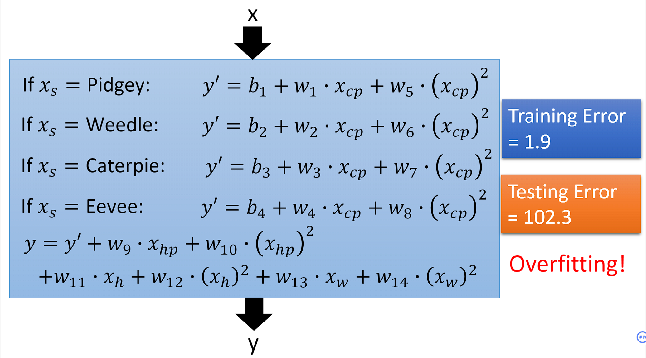
- When we don't just think about Pokémoncp值,Taking the species of Pokémon into account,The mean squared error on the test set is reduced to 14.3


- As we move on to consider other factors,Such as the height of each PokémonHeight,体重weight,经验值HP.The model becomes more complex at this point,Let's see how it performs on the test set,Very unfortunately the model overfits again.
3.5 正则化(Regularization)
为了解决过拟合的问题,We need to redesign the loss function L,The original loss function only calculated the variance,It does not take into account the influence of the input containing noise on the model.因此我们在 L Add an item after: λ ∑ ( w i ) 2 \lambda \sum (w_i)^2 λ∑(wi)2 ,This improves the generalization ability of the model,Make the model smoother,Reduce the sensitivity of the model to the input(Sensitive)
- Redesigned loss function L : L ( f ) = ∑ n ( y ^ n − ( b + ∑ w i x i ) ) 2 + λ ∑ ( w i ) 2 L(f)=\underset{n}{\sum}(\widehat{y}^n-(b+\sum w_ix_i))^2+\lambda \sum (w_i)^2 L(f)=n∑(yn−(b+∑wixi))2+λ∑(wi)2
Obviously according to the following experiment,We got better performance, 当 λ = 100 时, T e s t E r r o r = 11.1 当\lambda=100时,Test Error = 11.1 当λ=100时,TestError=11.1

边栏推荐
- TF中的条件语句;where()
- NTT的Another Me技术助力创造歌舞伎演员中村狮童的数字孪生体,将在 “Cho Kabuki 2022 Powered by NTT”舞台剧中首次亮相
- jar服务导致cpu飙升问题-带解决方法
- 【软件测试】(北京)字节跳动科技有限公司终面HR面试题
- prometheus学习5altermanager
- Discourse 的关闭主题(Close Topic )和重新开放主题
- prometheus学习4Grafana监控mysql&blackbox了解
- cdc连sqlserver异常对象可能有无法序列化的字段 有没有大佬看得懂的 帮忙解答一下
- 测试用例很难?有手就行
- 1002 Write the number (20 points)
猜你喜欢
【@网络工程师:用好这6款工具,让你的工作效率大翻倍!】
![[Recommender System]: Overview of Collaborative Filtering and Content-Based Filtering](/img/bc/fd2b8282269f460f4be2da78b84c22.png)
[Recommender System]: Overview of Collaborative Filtering and Content-Based Filtering
进制转换间的那点事

伦敦银规则有哪些?
机器学习总结(二)
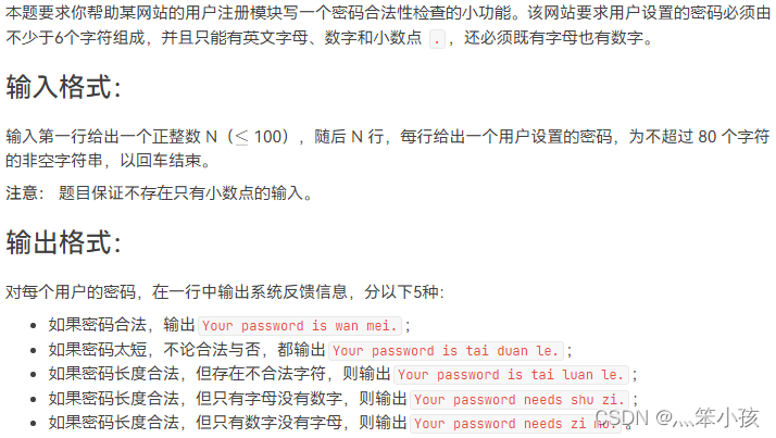
1081 检查密码 (15 分)

Implementation of FIR filter based on FPGA (5) - FPGA code implementation of parallel structure FIR filter
1081 Check Password (15 points)

接口测试的基础流程和用例设计方法你知道吗?
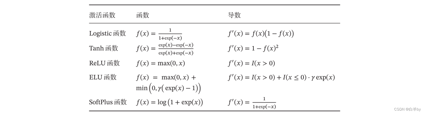
常见激活函数及其导数
随机推荐
1036 Programming with Obama (15 points)
Activity的四种启动模式
SQL滑动窗口
深度监督(中继监督)
语音信号处理:预处理【预加重、分帧、加窗】
1091 N-自守数 (15 分)
1056 组合数的和 (15 分)
1003 I want to pass (20 points)
js根据当天获取前几天的日期
TF通过feature与label生成(特征,标签)集合,tf.data.Dataset.from_tensor_slices
Redis源码:Redis源码怎么查看、Redis源码查看顺序、Redis外部数据结构到Redis内部数据结构查看源码顺序
机器学习总结(二)
你是如何做好Unity项目性能优化的
测试用例很难?有手就行
1.2-误差来源
Pinduoduo API interface
1071 Small Gamble (15 points)
1002 Write the number (20 points)
maxwell concept
1051 Multiplication of Complex Numbers (15 points)