当前位置:网站首页>Spark performance optimization guide
Spark performance optimization guide
2022-04-23 18:11:00 【Kungs8】
Catalog
- One 、 The basic chapter
-
- 1. Development tuning
-
- 1.1 Tuning Overview
- 1.2 Avoid creating duplicate RDD
- 1.3 Reuse the same... As much as possible RDD
- 1.4 For multiple use RDD persist
- 1.5 Avoid using shuffle Class operator
- 1.6 Use map-side Prepolymerized shuffle operation
- 1.7 Use high performance operators
- 1.8 Broadcast big variable
- 1.9 Use kryo Optimize serialization performance
- 1.10 Optimize data structure
- 2. Resource tuning
- Two 、 Advanced
-
- 1. Data skew
-
- 1.1 Tuning Overview
- 1.2 When data skew happens
- 1.3 How data skew happens
- 1.4 How to locate the code causing data skew
- 1.5 Data skew solution
-
- Scheme 1 : Use Hive ETL Preprocessing data
- Option two : Filtering a few causes tilting key
- Option three : Improve shuffle Parallelism of operations
- Option four : Two stage polymerization ( Local polymerization + Global aggregation )
- Option five : take reduce join To map join
- Programme 6 : Sampling tilt key And split up join operation
- Plan seven : Use random prefixes and resizing RDD Conduct join
- Plan 8 : Use a variety of options in combination
- 2. shuffle link
One 、 The basic chapter
In big data computing ,Spark It has become more and more popular 、 One of the more and more popular computing platforms .Spark The function of the system covers the off-line batch processing in the field of big data 、SQL Class processing 、 streaming / Real time computing 、 machine learning 、 Graph calculation and other different types of calculation operations , It has a wide range of applications and prospects . Many people have tried to use... In various projects Spark. majority ( Including me ), I started trying to use Spark The reason is simple , The main purpose is to make the execution speed of big data computing jobs faster 、 Higher performance .
However , adopt Spark Develop high performance big data computing jobs , It's not that simple . If there is no right Saprk The operation should be optimized reasonably ,Spark Job execution may be slow , In this way, there is no such thing as Spark The advantage of being a fast big data computing engine . So I want to make good use of it Spark, We must optimize its performance .
Spark Performance tuning is actually made up of many parts , It is not possible to improve the operation performance by adjusting several parameters . My mother needs different business scenarios and data , Yes Spark Make a comprehensive analysis of the work , Then adjust and optimize in many aspects , To get the best performance .
This is based on the previous Spark Job development experience and practice accumulation , Sum up a set of Spark Job performance optimization method . It is mainly divided into the following points : Development tuning 、 Resource tuning 、 Data skew tuning 、shuffle tuning These parts .
| Method | describe |
|---|---|
| Development tuning | all Spark Some basic principles to be paid attention to and followed in operation , It's high performance Spark The basis of the assignment |
| Resource tuning | all Spark Some basic principles to be paid attention to and followed in operation , It's high performance Spark The basis of the assignment |
| Data skew tuning | Used to solve Spark Solution to job data skew |
| shuffle tuning | Facing is right Spark People who have a deeper understanding and research of the principle . Mainly how to Saprk Operational shuffle Optimize the running process and details . |
Here is the basic chapter , It mainly focuses on analysis, development and resource tuning .
1. Development tuning
1.1 Tuning Overview
Spark The first step in performance optimization , Is to develop Spark Pay attention to and apply some basic principles of performance optimization in the process of operation . Development tuning , It is to let you know the following Spark Basic development principles :RDD lineage Design 、 Rational use of operators 、 Optimization of special operations, etc . In the development process , Always pay attention to the above principles , And these principles are based on the specific business and the actual application scenarios , Apply flexibly to your own Spark In homework .
1.2 Avoid creating duplicate RDD
Developing a Spark Homework time ,
1.  Based on a data source (eg: Hive Table or  HDFS file ) Create an initial RDD
2.  For this RDD Perform an operator operation , Get next RDD,
...( cycle , Know how to calculate the final result we want )
This process , Multiple RDD Will operate through different operators (eg: map、reduce etc. ) String together , This "RDD strand " Namely RDD lineage, That is to say “RDD The chain of consanguinity ”.
Be careful : For the same data , Only one... Should be created RDD, Cannot create more than one RDD To represent the same data .
some Spark Beginners are just starting to develop Spark Homework time , Or experienced engineers are developing RDD lineage Extremely lengthy Spark Homework time , You may forget that you have created a for a piece of data before RDD, This leads to the same data , Created multiple RDD, That means ,Spark The job performs multiple iterations to create multiple... That represent the same data RDD, In turn, the performance overhead of the job is added .
A simple example :
//  It needs to be called “hello.txt” Of HDFS File once map operation , Do it again reduce operation . in other words , You need to perform two operator operations on a piece of data .

// 1.  Wrong way : When performing multiple operator operations on the same data , Create multiple RDD.
//  It's done here twice textFile Method , For the same HDFS file , I created two RDD come out , And then separately for each RDD All perform an operator operation .
//  In this case ,Spark Need from HDFS Last two loads hello.txt The content of the document , And create two separate RDD; Second load HDFS File and create RDD Performance overhead , It's obviously wasted .
val rdd1 = sc.textFile("hdfs://192.168.0.1:9000/hello.txt")
rdd1.map(...)
val rdd2 = sc.textFile("hdfs://192.168.0.1:9000/hello.txt")
rdd2.reduce(...)

// 2.  The right way to use : When performing multiple operator operations on a piece of data , Use only one RDD.
//  This style of writing is obviously much better than the previous one , Because we only create one... For the same data RDD, And then to this one RDD Multiple operator operations performed .
//  But notice that optimization is not over yet , because rdd1 Operator operations are performed twice , Second execution reduce During operation , It will be recalculated again from the source rdd1 The data of , So there is still the performance overhead of double counting .
//  To solve this problem thoroughly , Must be combined with “ Principle three : For multiple use RDD persist ”, To guarantee a RDD When used multiple times, it is calculated only once .
val rdd1 = sc.textFile("hdfs://192.168.0.1:9000/hello.txt")
rdd1.map(...)
rdd1.reduce(...)
1.3 Reuse the same... As much as possible RDD
In addition to avoiding creating more than one piece of identical data during the development process RDD outside , When performing operator operations on different data, try to reuse one as much as possible RDD. for instance , There is one RDD The data format of is key-value Type of , The other is Shan value Type of , these two items. RDD Of value The data is exactly the same . Then we can only use key-value The type of RDD, Because it already contains another piece of data . For many like this RDD There are overlaps or inclusions in the data of , We should try to reuse one RDD, This can reduce... As much as possible RDD The number of , So as to minimize the number of times the operator executes .
A simple example :
// 1.  Wrong way .

//  There is one <Long, String> Format RDD, namely rdd1.
//  Then because of business needs , Yes rdd1 Executed a map operation , Created a rdd2, and rdd2 The data in is just rdd1 Medium value It's just worth it , in other words ,rdd2 yes rdd1 Subset .
JavaPairRDD<Long, String> rdd1 = ...
JavaRDD<String> rdd2 = rdd1.map(...)

//  Respectively for rdd1 and rdd2 Different operator operations are performed .
rdd1.reduceByKey(...)
rdd2.map(...)

// 2.  The right way .

//  Above this case in , Actually rdd1 and rdd2 The difference is nothing more than data format ,rdd2 The data of is exactly rdd1 It's just a subset of , But created two rdd, And for two rdd All performed an operator operation .
//  At this time, it will be because of the right rdd1 perform map Operator to create rdd2, And one more operator operation , This in turn increases performance overhead .

//  In fact, in this case, you can reuse the same RDD.
//  We can use rdd1, Do both reduceByKey operation , Also do map operation .
//  In the second map In operation , Use only... For each data tuple._2, That is to say rdd1 Medium value value , that will do .
JavaPairRDD<Long, String> rdd1 = ...
rdd1.reduceByKey(...)
rdd1.map(tuple._2...)

//  The second way is compared with the first way , It's obviously reduced once rdd2 The cost of Computing .
//  But so far , Optimization is not over yet , Yes rdd1 We still do two operator operations ,rdd1 In fact, it will be calculated twice .
//  So we need to cooperate with “ For multiple use RDD persist ” To use , To guarantee a RDD When used multiple times, it is calculated only once .
1.4 For multiple use RDD persist
When you are in Spark Multiple times in the code for one RDD After doing the operator operation , Congratulations , You have achieved Spark Optimization of the first step of the assignment , That is, reuse as much as possible RDD. It's time to build on that , The second step is to optimize , That's to make sure that you're right RDD When performing multiple operator operations , This RDD Itself is only counted once .
Spark For one RDD The default principle for performing multiple operators is : Every time you talk to one RDD When performing an operator operation , It will be recalculated from the source , Work out the RDD Come on , And then to this RDD Perform your operator operations . The performance of this method is very poor .
So in this case , Our suggestion is : For multiple use RDD persist . here Spark According to your persistence strategy , take RDD The data in is saved to memory or disk . Every time after that RDD When doing operator operations , Will extract persistence directly from memory or disk RDD data , And then the operator , Instead of recalculating this from the source RDD, Then perform the operator operation .
A simple example :df.persist(pyspark.StorageLevel.MEMORY_AND_DISK_SER)
//  If there is to be a RDD persist , Just for this RDD call cache() and persist() that will do .

//  The right way .
// cache() Method representation : Use non serialization to RDD All the data in are trying to persist into memory .
//  Right now rdd1 When performing two operator operations , Only for the first time map Operator time , That's what makes this rdd1 Once from the source .
//  Second execution reduce Operator time , It will extract data directly from memory for calculation , There is no double counting of rdd.
val rdd1 = sc.textFile("hdfs://192.168.0.1:9000/hello.txt").cache()
rdd1.map(...)
rdd1.reduce(...)

// persist() Method representation : Select the persistence level manually , And persist in the specified way .
//  for instance ,StorageLevel.MEMORY_AND_DISK_SER Express , When enough memory is available, it is preferred to persist in memory , Persist to disk file when memory is not enough .
//  And one of them _SER postfix notation , Use serialization to save RDD data , here RDD Each of the partition Will be sequenced into a large byte array , Then persist to memory or disk .
//  Serialization can reduce the persistence of data on memory / Disk usage , In this way, the memory is not used too much by persistent data , It happens frequently GC.
val rdd1 = sc.textFile("hdfs://192.168.0.1:9000/hello.txt").persist(StorageLevel.MEMORY_AND_DISK_SER)
rdd1.map(...)
rdd1.reduce(...)
about persist() In terms of method , We can choose different persistence levels according to different business scenarios .
Spark The persistence level of
| Persistence level | Explanation of meaning |
|---|---|
| MEMORY_ONLY | The default option ,RDD Of ( Partition ) The data is directly expressed as Java The form of an object is stored in JVM The memory of the , If there's not enough memory , The data of some partitions will not be cached , It needs to be recalculated according to the generation information when using . This is the default persistence strategy , Use cache() When the method is used , This is actually the persistence strategy used . |
| MYMORY_AND_DISK | RDD The data is directly in Java The form of an object is stored in JVM The memory of the , If the memory space is not , The data of some partitions will be stored on disk , Read from disk when using |
| MEMORY_ONLY_SER | RDD The data of (Java object ) After serialization, it is stored in JVM The memory of the ( The data of a partition is a byte array in memory ), Compared with MEMORY_ONLY It can effectively save memory space ( Especially when using a fast serialization tool ), But more time is needed to read the data CPU expenses ; If there's not enough memory , How to deal with MEMORY_ONLY identical . |
| MEMORY_AND_DISK_SER | Compared with MEMORY_ONLY_SER, In case of insufficient memory space , Store the serialized data on disk . |
| DISK_ONLY | Use only disk storage RDD The data of ( Not serialized ). |
| MEMORY_ONLY_2,MEMORY_AND_DISK_2, etc. | For any of the above persistence strategies , If you add a suffix ‘_2’, It's about persisting every piece of data , Make a copy of it , And save the copy to other nodes , This replica based persistence mechanism is mainly used for fault tolerance . If a node hangs up , Persistent data in the node's memory or disk is lost , Then the follow-up is right RDD Copies of the data on other nodes can also be used for calculation ; If there is no copy , The guide recalculates these data from the source . |
| OFF_HEAP(experimental) | OFF_HEAP(experimental) RDD The data is stored in... After being instantiated Tachyon. Compared with MEMORY_ONLY_SER,OFF_HEAP Can reduce garbage collection costs 、 bring Spark Executor more “ Small ” more “ light ” Can share memory at the same time ; And the data is stored in Tachyon in ,Spark Cluster node failure does not cause data loss , So in this way “ Big ” It is very attractive in the scenario of memory or multiple concurrent applications . It should be noted that ,Tachyon Not directly included in Spark Within the system of , You need to select the appropriate version for deployment ; Its data is based on “ block ” Managing for the unit , These blocks can be discarded according to a certain algorithm , And will not be rebuilt |
How to choose the most appropriate persistence strategy
By default , Of course, the highest performance is MEMORY_ONLY, But only if you have enough memory , More than enough to store the whole RDD All data for . Because there is no serialization or deserialization , This part of the performance overhead is avoided ; For this RDD The subsequent operator operations of , All operations are based on data in pure memory , There is no need to read data from the disk file , High performance ; And there's no need to make a copy of the data , And remote transmission to other nodes . But what we have to pay attention to here is , In the actual production environment , I'm afraid there are limited scenarios where this strategy can be used directly , If RDD When there are more data in ( For example, billions ), Use this persistence level directly , It can lead to JVM Of OOM Memory overflow exception .
If you use MEMORY_ONLY Memory overflow at level , So it is recommended to try to use MEMORY_ONLY_SER Level . This level will RDD Data is serialized and stored in memory , At this point, each of them partition It's just an array of bytes , It greatly reduces the number of objects , And reduce the memory consumption . This is a level ratio MEMORY_ONLY Extra performance overhead , The main thing is the cost of serialization and deserialization . But subsequent operators can operate based on pure memory , So the overall performance is relatively high . Besides , The possible problems are the same as above , If RDD If there is too much data in , Or it may lead to OOM Memory overflow exception .
If the level of pure memory is not available , Then it is recommended to use MEMORY_AND_DISK_SER Strategy , instead of MEMORY_AND_DISK Strategy . Because now that it's this step , Just explain RDD A lot of data , Memory can't be completely down . The serialized data is less , Can save memory and disk space overhead . At the same time, this strategy will try to cache data in memory as much as possible , Write to disk if memory cache is not available .
It is generally not recommended to use DISK_ONLY And suffixes are ’_2’ The level of : Because the data is read and write based on the disk file , Can cause a dramatic performance degradation , Sometimes it's better to recalculate all RDD. The suffix is ’_2’ The level of , All data must be copied in one copy , And send it to other nodes , Data replication and network transmission will lead to large performance overhead , Unless high availability of the job is required , Otherwise, it is not recommended to use .
1.5 Avoid using shuffle Class operator
If possible , Try to avoid using shuffle Class operator . because Spark During job operation , The most performance consuming part is shuffle The process .shuffle The process , Simply speaking , It is the same node distributed in the cluster key, Pull to the same node , To aggregate or join Wait for the operation . such as reduceByKey、join Equal operator , Will trigger shuffle operation .
shuffle In the process , The same on each node key Will be written to the local disk file first , Then other nodes need to pull the same disk file on each node through network transmission key. And the same key When you take the same node for aggregation operation , It may also be because of the key Too much , Cause insufficient memory , And then overflow to the disk file . So in shuffle In the process , There may be a lot of reading and writing of disk files IO operation , And data network transmission operation . disk IO And network data transmission shuffle The main reason for poor performance .
So in our development process , Avoid using if possible reduceByKey、join、distinct、repartition We'll do it later shuffle The operator of , Use as much as possible map Class's non shuffle operator . In this case , No, shuffle Operation or less shuffle Operation of the Spark Homework , Can greatly reduce performance overhead .
Broadcast And map Conduct join Code example
//  Conventional join The operation will cause shuffle operation .
//  Because the two one. RDD in , same key All need to be pulled to a node through the network , By a task Conduct join operation .
val rdd3 = rdd1.join(rdd2)

// Broadcast+map Of join operation , Will not lead to shuffle operation .
//  Use Broadcast Put a small amount of data RDD As a broadcast variable .
val rdd2Data = rdd2.collect()
val rdd2DataBroadcast = sc.broadcast(rdd2Data)

//  stay rdd1.map In operator , It can be downloaded from rdd2DataBroadcast in , obtain rdd2 All data for .
//  And then we're going to iterate , If you find that rdd2 Of a piece of data key And rdd1 Of the current data key It's the same , Then it can be judged that join.
//  At this time, you can according to your own needs , take rdd1 Current data and rdd2 Data that can be connected in , Splice together (String or Tuple).
val rdd3 = rdd1.map(rdd2DataBroadcast...)

//  Be careful , The above operation , The advice is only in rdd2 The amount of data is relatively small ( For example, hundreds of M, Or one or two G) In case of use .
//  Because of every Executor The memory of the , There will always be one rdd2 The full amount of data .
1.6 Use map-side Prepolymerized shuffle operation
If it's because of business needs , Be sure to use shuffle operation , No use map Class to replace , Then try to use it map-side Prepolymerization operators .
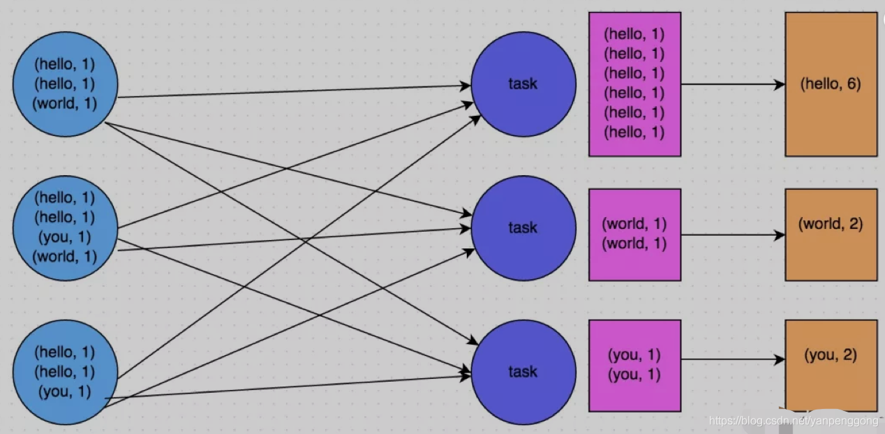
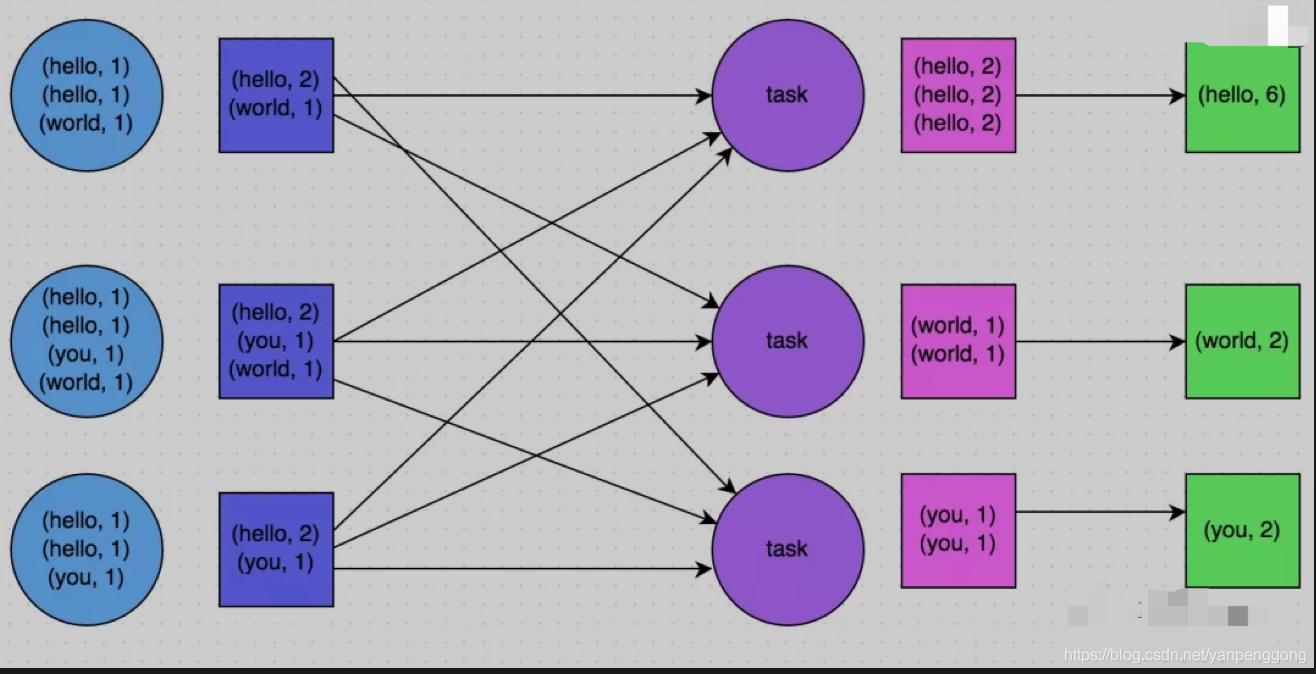
So-called map-side Prepolymerization , It is said that each node is local to the same key Do an aggregate operation , Be similar to MapReduce Local in combiner.map-side After prepolymerization , Each node will have only one local key, Because many of the same key It's all converged . Other nodes are the same in pulling all nodes key when , It will greatly reduce the amount of data to be pulled , This reduces the number of disks IO And network transmission overhead . Generally speaking , Where possible , It is recommended to use reduceByKey perhaps aggregateByKey Operator to replace groupByKey operator . because reduceByKey and aggregateByKey Operators will use user-defined functions for each node local to the same key Prepolymerization . and groupByKey Operators are not prepolymerized , The full amount of data will be distributed and transmitted among the nodes of the cluster , Relatively poor performance .
For example, the following two pictures , It's a typical example , Based on reduceByKey and groupByKey Count the words . The first picture is groupByKey The schematic diagram of , You can see , When there is no local aggregation , All data is transferred between cluster nodes ; The second picture is reduceByKey The schematic diagram of , You can see , Each node is the same locally key data , It's all prepolymerized , Then it is transferred to other nodes for global aggregation .
1.7 Use high performance operators
except shuffle Related operators have optimization principles , Other operators also have corresponding optimization principles .
- Use reduceByKey/aggregateByKey replace groupByKey
For details, see “ Use map-side Prepolymerized shuffle operation ”. - Use mapPartitions Replace the common map
mapPartitions Class operator , A function call will handle one partition All data , Instead of processing one function call at a time , Relatively high performance . But sometimes , Use mapPartitions There will be OOM( out of memory ) The problem of . Because a single function call has to deal with one partition All data , If there's not enough memory , Too many objects can't be recycled in garbage collection , It's possible that OOM abnormal . So be careful when using this kind of operation ! - Use foreachPartitions replace foreach
The principle is similar to “ Use mapPartitions replace map”, It's also a function call to handle one partition All data for , Instead of processing a piece of data with a function call . It is found in practice that ,foreachPartitions Class operator , It's very helpful to improve the performance . For example foreach Function , take RDD All data in write MySQL, So if it's ordinary foreach operator , It will write data by data , Each function call may create a database connection , At this point, the database connection will be created and destroyed frequently , Performance is very low ; But if you use foreachPartitions The operator processes one at a time partition The data of , So for each partition, Just create a database connection , Then perform the bulk insert operation , At this time, the performance is relatively high . Found in practice , about 1 About ten thousand pieces of data are measured and written MySQL, Performance can be improved 30% above . - Use filter after coalesce operation
Usually for a RDD perform filter Operator filters out RDD After more data ( such as 30% The above data ), It is recommended to use coalesce operator , Manual reduction RDD Of partition Number , take RDD The data in is compressed to less partition In the middle . because filter after ,RDD Each partition There will be a lot of data filtered out , At this time, if the subsequent calculation is carried out as usual , In fact, each of them task To deal with the partition Not a lot of data in , A little waste of resources , And it's dealt with at this time task The more , Maybe the slower the speed is . So with coalesce Reduce partition Number , take RDD The data in is compressed to less partition after , Just use less task You can handle everything partition. In some cases , It will help to improve the performance . - Use repartitionAndSortWithinPartitions replace repartition And sort Class action
repartitionAndSortWithinPartitionsyes Spark An operator recommended by the official website , The official advice , If you need to repartition After repartition , And sort it out , Recommended direct userepartitionAndSortWithinPartitionsoperator . Because this operator can do the partition at the same time shuffle operation , Sort at the same time .shuffle And sort Two operations at the same time , Before shuffle Again sort Come on , Performance may be high .
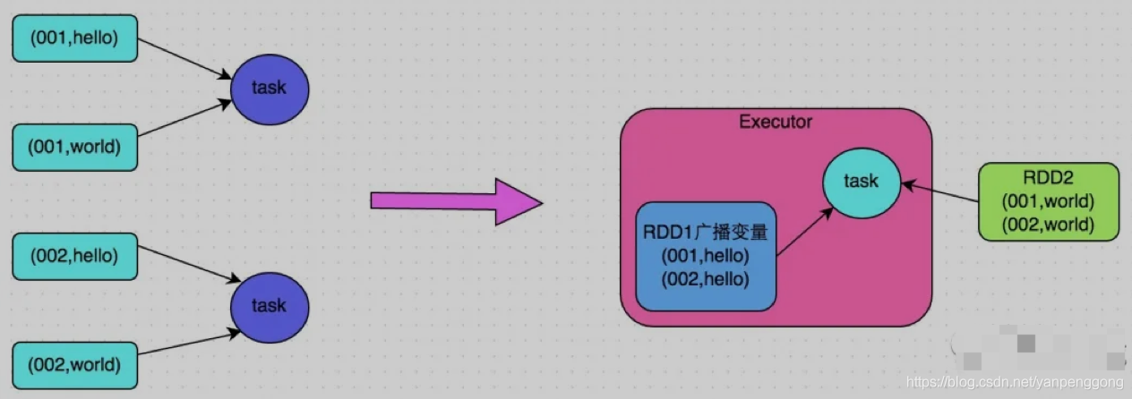
1.8 Broadcast big variable
Sometimes in the development process , You will encounter scenarios where you need to use external variables in operator functions ( Especially large variables , such as 100M The collection of the above ), Then you should use Spark Broadcast of (Broadcast) Features to improve performance .
When external variables are used in operator functions , By default ,Spark Multiple copies of this variable will be copied , To transmit over a network to task in , At this point, each of them task All have a copy of the variable . If the variable itself is large ( such as 100M, even to the extent that 1G), So the performance overhead of a large number of variable copies transmitted in the network , And at each node Executor Too much memory is used in GC, Will greatly affect performance .
So for the above , If the external variables used are large , It is recommended to use Spark The broadcast function of , Broadcast this variable . Variables after broadcast , Will guarantee that each Executor The memory of the , Only one copy of the variable resides , and Executor Medium task Share the Executor The copy of the variable in . In this case , Can greatly reduce the number of variable copies , So as to reduce the performance overhead of network transmission , And reduce the Executor Memory usage cost , Reduce GC The frequency of .
Code example of broadcast big variable
//  The following code is in the operator function , Using external variables .
//  There is no special operation at this time , Every task There will be a copy list1 Copy of .
val list1 = ...
rdd1.map(list1...)

//  The following code will list1 Encapsulation is Broadcast Type of broadcast variable .
//  In the operator function , When using broadcast variables , First of all, it will judge the current task Where Executor In the memory , Are there copies of variables .
//  If so, use ; If not, from Driver Or other Executor Pull a remote copy from the node and put it in the local area Executor In the memory .
//  Every Executor In the memory , Only one copy of the broadcast variables will reside .
val list1 = ...
val list1Broadcast = sc.broadcast(list1)
rdd1.map(list1Broadcast...)
1.9 Use kryo Optimize serialization performance
stay Spark in , There are three main areas of serialization :
- When external variables are used in operator functions , This variable will be serialized for network transmission ( see “1.8 Broadcast big variable ” Explanation in ).
- Use the custom type as RDD The generic type of ( such as JavaRDD,Student It's a custom type ), All custom type objects , Will be serialized . So in this case , It also requires that the custom class must implement Serializable Interface .
- When using serializable persistence policies ( such as MEMORY_ONLY_SER),Spark Will RDD Each of the partition Are sequenced into a large array of bytes .
For these three places where serialization occurs , We can all use Kryo Serialization class library , To optimize the performance of serialization and deserialization .Spark The default is Java The serialization mechanism of , That is to say ObjectOutputStream/ObjectInputStream API To serialize and deserialize . however Spark It also supports the use of Kryo Serialization Library ,Kryo Performance ratio of serialization class library Java The performance of serialization class library is much higher . The official introduction ,Kryo Serialization mechanism Java Serialization mechanism , High performance 10 About times .Spark The reason why it is not used by default Kryo As a serialization class library , Because Kryo It's best to register all custom types that need to be serialized , So for developers , This way is more troublesome .
Here are the USES Kryo Code example of , We just need to set the serialization class , Then register the custom type to be serialized ( For example, the types of external variables used in operator functions 、 As RDD Custom types of generic types, etc ):
//  establish SparkConf object .
val conf = new SparkConf().setMaster(...).setAppName(...)
//  Set the serializer to KryoSerializer.
conf.set("spark.serializer", "org.apache.spark.serializer.KryoSerializer")
//  Register custom types to serialize .
conf.registerKryoClasses(Array(classOf[MyClass1], classOf[MyClass2]))
1.10 Optimize data structure
Java in , There are three types of memory consumption :
- object , Every Java Objects all have object heads 、 Quotes and other additional information , So it takes up more memory .
- character string , Inside each string there is an array of characters and extra information such as length .
- Collection types , such as HashMap、LinkedList etc. , Because collection types usually use some inner classes to encapsulate collection elements , such as Map.Entry.
therefore Spark The official advice , stay Spark Coding implementation , Especially for the code in the operator function , Try not to use these three data structures , Try to use strings instead of objects , Use original type ( such as Int、Long) Alternative string , Use arrays instead of collection types , This reduces the memory footprint as much as possible , To reduce GC frequency , Lifting performance .
But in the author's coding practice, I found that , It's not easy to do that . Because we also need to consider the maintainability of the code , If in a code , There is no object abstraction at all , It's all string splicing , So for subsequent code maintenance and modification , There is no doubt that it is a great disaster . Empathy , If all operations are based on arrays , Instead of using HashMap、LinkedList And so on , So for our coding difficulty and code maintainability , It's also a great challenge . So I suggest , Where possible and appropriate , Use a data structure that uses less memory , But the premise is to ensure the maintainability of the code .
2. Resource tuning
2.1 Tuning Overview
At the end of development Spark After the homework , It's time to allocate the right resources for the job .Spark Resource parameters for , Almost all of them can be found in spark-submit Set as a parameter in the command . quite a lot Spark beginner , Usually I don't know what necessary parameters to set , And how to set these parameters , In the end, you can only set it up randomly , Not even at all . Unreasonable setting of resource parameters , It may lead to underutilization of cluster resources , Jobs run extremely slowly ; Or the set resource is too large , The queue does not have enough resources to provide , And then lead to all kinds of abnormalities . All in all , Either way , Will result in Spark The operation of the job is inefficient , It doesn't even work . So we have to be right about Spark There is a clear understanding of the principle of resource use of homework , And know that in Spark During job operation , Which resource parameters can be set , And how to set the appropriate parameter value .
2.2 Spark Basic operation principle of the job
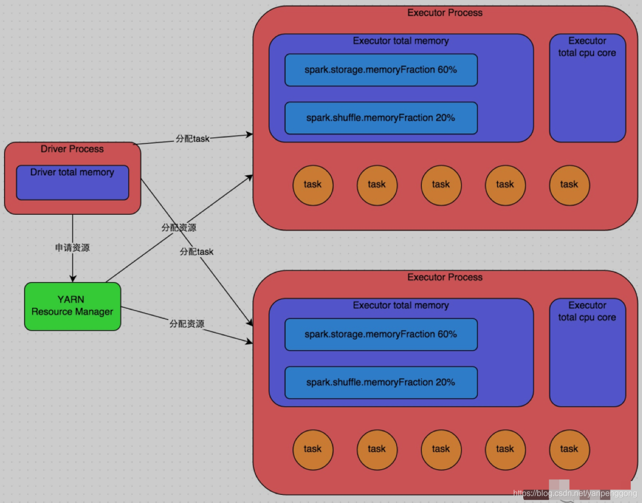
The detailed principle is shown in the figure above . We use spark-submit To submit a Spark After the homework , This job will start a corresponding Driver process . According to the deployment mode you use (deploy-mode) Different ,Driver The process may start locally , It is also possible to start on a working node in the cluster .Driver The process itself will be based on the parameters we set , Occupy a certain amount of memory and CPU core. and Driver The first thing the process needs to do , To cluster manager ( It can be Spark Standalone colony , It can also be another resource management cluster , What we use here is YARN As a resource management cluster ) Apply to run Spark Resources needed for the job , The resources here refer to Executor process .YARN The cluster manager will follow us for Spark Resource parameters for job settings , On each work node , Start a certain number of Executor process , Every Executor Processes all occupy a certain amount of memory and CPU core.
After applying for the resources needed for job execution ,Driver The process will start to schedule and execute the job code we wrote .Driver The process will write Spark The job code is split into multiple stage, Every stage Execute some code snippets , And for each stage Create a batch of task, And then put these task Assign to each Executor In process execution .task It's the smallest computing unit , As like as two peas ( That's a piece of code we wrote ourselves ), Just every one task The data is different . One stage All of the task When it's all done , The calculation intermediate result will be written in the local disk file of each node , then Driver Will schedule the next stage. next stage Of task The input data of is the last one stage The intermediate result of the output . And so on and so on , Until the logic of our own code is completely executed , And calculate all the data , Until we get what we want .
Spark It's based on shuffle Class operators stage Division . If we execute something in our code shuffle Class operator ( such as reduceByKey、join etc. ), So it's going to be at this operator , Divide up a stage Boundaries come . It can be roughly understood as ,shuffle Before the operator executes, the code will be divided into stage,shuffle Operator execution and subsequent code will be divided into the next stage. So a stage At the beginning of execution , Each of them task Probably all from the last stage Of task The node , To pull all the things that need to be handled by oneself through network transmission key, And then pull all the same key Use our own operator functions to perform aggregation operations ( such as reduceByKey() Function received by operator ). This process is shuffle.
When we execute in code cache/persist Wait for the persistence operation , Depending on the persistence level we choose , Every task The calculated data will also be saved to Executor The memory of the process or the disk file of the node .
therefore Executor The main memory is divided into three parts :
- The first is to let task Use... When executing our own code , The default is to occupy Executor Total memory 20%;
- The second is to let task adopt shuffle The process takes the last stage Of task After the output of , Used for polymerization and other operations , Default is also accounted for Executor Total memory 20%;
- The third is to let RDD Use... For persistence , Default occupation Executor Total memory 60%.
task The execution speed of each Executor Process CPU core Quantity has a direct bearing on . One CPU core Only one thread can be executed at a time . And each Executor More than one... Assigned to a process task, With each task The way a thread works , Multithreading runs concurrently . If CPU core There are plenty of them , And assigned to task The quantity is reasonable , So usually , This can be done quickly and efficiently task Threads .
That's all Spark Description of the basic operation principle of the job , You can use the above picture to understand . Understand the basic principles of operation , It is the basic premise of resource parameter tuning .
2.3 Resource parameter tuning
Understand the finished Spark After the basic principle of job operation , Parameters related to resources are easy to understand . So-called Spark Resource parameter tuning , In fact, it's mainly right Spark Where resources are used during the operation , By adjusting various parameters , To optimize the efficiency of resource utilization , Thus enhance Spark Performance of the job . The following parameters are Spark The main resource parameters in , Each parameter corresponds to a part of the job's operation principle , We also give a reference value for tuning .
1. num-executors
Parameter description : This parameter is used to set Spark How many homework do you need in total Executor Process to execute .Driver In the YARN When the cluster manager requests resources ,YARN The cluster manager will try to follow your settings on the working nodes of the cluster , Start the corresponding number of Executor process . This parameter is very important , If not set , By default, only a small amount of Executor process , Your Spark The job runs very slowly .
Parameter tuning suggestions : Every Spark General settings of job operation 50~100 About Executor The process is more appropriate , Too few or too many settings Executor The process is not good . Too few settings , Can't make full use of cluster resources ; If there are too many settings , Most queues may not be able to give sufficient resources .
2. executor-memory
Parameter description : This parameter is used to set each Executor Process memory .Executor Memory size , A lot of times it's a direct decision Spark Performance of the job , And with the common JVM OOM abnormal , There's also a direct connection .
Parameter tuning suggestions : Every Executor Memory settings for processes 4G (8G A more appropriate . But it's just a reference value , The specific settings should be determined according to the resource queues of different departments . You can see the maximum memory limit of your team's resource queue ,num-executors multiply executor-memory, Can't exceed the maximum amount of memory in the queue . Besides , If you are sharing this resource queue with others in the team , Then the amount of memory requested should not exceed the maximum total memory of the resource queue 1/3)1/2, Avoid your own Spark The job takes up all the resources of the queue , Cause other students' homework can't run .
3. executor-cores
Parameter description : This parameter is used to set each Executor Process CPU core Number . This parameter determines each Executor Process execution in parallel task The ability of threads . Because of every CPU core Only one... Can be executed at a time task Threads , So every Executor Process CPU core The more the number of , The more quickly you can execute all of the things that are assigned to you task Threads .
Parameter tuning suggestions :Executor Of CPU core The quantity is set to 2~4 One is more suitable . It also depends on the resource queue of different departments , You can see the largest resource queue of your own CPU core What is the limit , Then according to the setting Executor Number , To decide on each Executor Processes can be assigned to several CPU core. It is also suggested that , If you are sharing this queue with others , that num-executors * executor-cores Don't exceed the queue total CPU core Of 1/3~1/2 Right or left , It is also to avoid affecting the operation of other students' homework .
4. driver-memory
Parameter description : This parameter is used to set Driver Process memory .
Parameter tuning suggestions :Driver The memory of is usually not set , Or set up 1G Left and right should be enough . The only thing to notice is , If needed collect Operator will RDD Pull all the data to Driver Top processing , Then you have to make sure that Driver The memory is big enough , Otherwise OOM Memory overflow problem .
5. spark.default.parallelism
Parameter description : This parameter is used to set each stage Default task Number . This parameter is very important , If you don't set it, it may directly affect your Spark Performance .
Parameter tuning suggestions :Spark Default for homework task The number of 500~1000 One is more suitable . A common mistake many students make is not to set this parameter , Then it will lead to Spark According to the bottom HDFS Of block Quantity to set task The number of , The default is a HDFS block Corresponding to one task. Generally speaking ,Spark The number of default settings is too small ( For example, dozens of task), If task If the quantity is too small , It will cause you to set up the Executor All the parameters of are wasted . Just imagine , Whatever you are Executor How many processes , Memory and CPU How big is the , however task Only 1 A or 10 individual , that 90% Of Executor The process may not have task perform , It's a waste of resources ! therefore Spark The setting principle recommended by the official website is , Set the parameter to num-executors * executor-cores Of 2~3 Times more appropriate , such as Executor Total CPU core The number of 300 individual , Then set 1000 individual task Yes. , We can make full use of Spark Cluster resources .
6. spark.storage.memoryFraction
Parameter description : This parameter is used to set RDD Persistent data in Executor The percentage of memory that can be used , The default is 0.6. in other words , Default Executor 60% Of memory , Can be used to save persistent RDD data . Depending on the persistence strategy you choose , If there is not enough memory , Maybe the data won't last , Or data will be written to disk .
Parameter tuning suggestions : If Spark In homework , There are more RDD Persistence operation , The value of this parameter can be increased a little bit , Ensure that persistent data can be stored in memory . Avoid not having enough memory to cache all the data , Causes data to be written only to disk , Reduced performance . But if Spark In homework shuffle Class operations are more , And the persistence operation is less , So it's better to reduce the value of this parameter . Besides , If it is found that the work is due to frequent gc Causes slow operation ( adopt spark web ui You can observe the homework gc Time consuming ), signify task Not enough memory to execute user code , It is also recommended to lower the value of this parameter .
7. spark.shuffle.memoryFraction
Parameter description : This parameter is used to set shuffle In the process a task Pull to the last stage Of task After the output of , Can be used for aggregation operations Executor The proportion of memory , The default is 0.2. in other words ,Executor Only by default 20% Memory for this operation .shuffle The operation is in the process of aggregation , If you find that you are using more memory than this 20% The limitation of , Then the redundant data will overflow to the disk file , At this point, the performance will be greatly reduced .
Parameter tuning suggestions : If Spark In homework RDD Less persistence ,shuffle When there are many operations , It is recommended to reduce the memory share of persistent operations , Improve shuffle The proportion of operation memory , avoid shuffle When there is too much data in the process, the memory is not enough , Must overflow to disk , Reduced performance . Besides , If it is found that the work is due to frequent gc Causes slow operation , signify task Not enough memory to execute user code , It is also recommended to lower the value of this parameter . Tuning of resource parameters , There is no fixed value , Need students according to their actual situation ( Include Spark In homework shuffle Number of operations 、RDD The number of persistence operations and spark web ui The assignments shown in gc situation ), At the same time, refer to the principles and tuning suggestions given in this article , Set the above parameters reasonably .
Resource parameter reference example
Here is a copy of spark-submit Examples of commands , You can refer to it , And according to their own actual situation to adjust :
./bin/spark-submit \
  --master yarn-cluster \
  --num-executors 100 \
  --executor-memory 6G \
  --executor-cores 4 \
  --driver-memory 1G \
  --conf spark.default.parallelism=1000 \
  --conf spark.storage.memoryFraction=0.5 \
  --conf spark.shuffle.memoryFraction=0.3 \
According to practical experience , Most of the Spark After the development tuning and resource tuning explained in this basic chapter , Generally, it can run with high performance , Enough to meet our needs . But in different production environments and project contexts , There may be other, more intractable problems ( For example, all kinds of data skew ), There may also be higher performance requirements . To meet these challenges , More advanced techniques are needed to deal with such problems .
Two 、 Advanced
1. Data skew
1.1 Tuning Overview
sometimes , We may encounter one of the most difficult problems in big data calculation —— Data skew , here Spark The performance of the job will be much worse than expected . Data skew tuning , It is to use various technical solutions to solve different types of data skew problems , In order to make sure Spark Performance of the job .
1.2 When data skew happens
- most task It's very fast , But individually task Very slow execution . such as , All in all 1000 individual task,997 individual task All in 1 It's done in minutes , But there are two or three left task But it will take an hour or two . This is very common .
- What could have been performed normally Spark Homework , One day suddenly reported OOM( out of memory ) abnormal , Observe the exception stack , It's the business code we wrote that caused . This is rare .
1.3 How data skew happens
The principle of data skew is very simple : It's going on shuffle When , You must set the same... On each node key Pull to a node task To process , For example, according to key To aggregate or join Wait for the operation . At this point, if some key If the corresponding amount of data is very large , Data skew happens . For example, most of key Corresponding 10 Data , But individually key But it corresponds to 100 Ten thousand data , So most of it task Maybe it will only be allocated to 10 Data , then 1 In seconds ; But individually task May have been assigned to 100 All the data , It's going to run for an hour or two . therefore , Whole Spark The running progress of the job is determined by the one with the longest running time task Decisive .
So when data skews ,Spark Jobs seem to run very slowly , Maybe even because of some task The amount of data processed is too large, resulting in memory overflow .
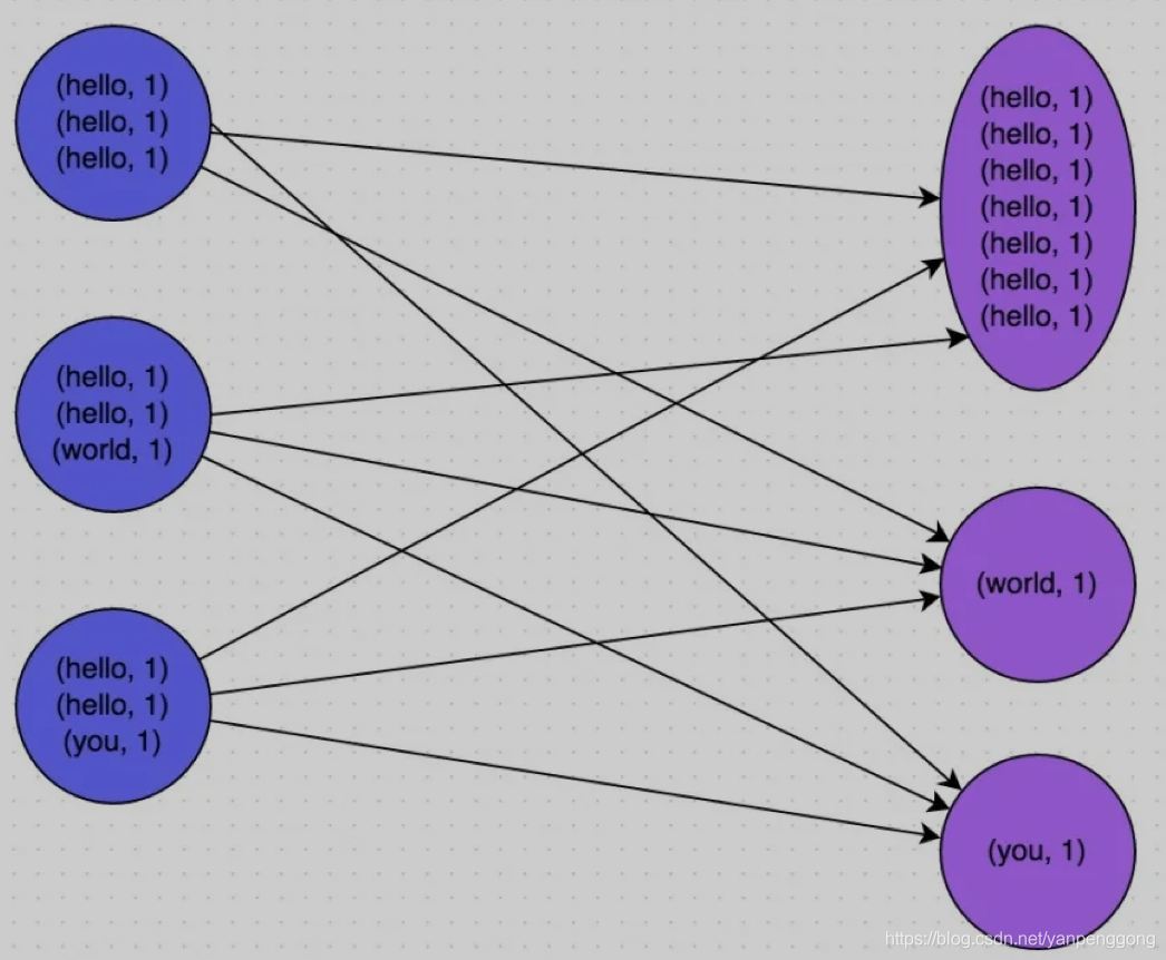
The picture below is a very clear example :hello This key, There are three nodes corresponding to a total of 7 Data , All these data will be pulled to the same task Intermediate processing ; and world and you these two items. key The difference corresponds to 1 Data , So the other two task Just deal with it separately 1 Data . The first one at this time task The run time of may be the other two task Of 7 times , And the whole stage And the slowest one task Determined by .
1.4 How to locate the code causing data skew
Data skew only happens in shuffle In the process . Here's a list of common ones that may trigger shuffle Operator of operation :distinct、groupByKey、reduceByKey、aggregateByKey、join、cogroup、repartition etc. . When data skews , Maybe it's the result of using one of these operators in your code .
1.4.1 Some task A situation in which execution is particularly slow
The first thing to see is , It's the data skew that happens in the first few stage in .
If it is to use yarn-client Mode submission , Then you can see it directly here log Of , Can be in log Found the current run to the next few stage; If it is to use yarn-cluster Mode submission , You can use the Spark Web UI To see how many are currently running stage. Besides , Whether to use yarn-client Mode or yarn-cluster Pattern , We can all be in Spark Web UI Take a deep look at the current stage each task The amount of data allocated , So as to further determine whether it is task Uneven distribution of data results in data skew .
As shown in the picture below , The third to last column shows each task Running time of . You can clearly see that , yes , we have task Very fast , It only takes a few seconds to run ; Others task It's very slow , It will take a few minutes to run , At this time, the data skew can be determined from the running time alone . Besides , The first to last column shows each task The amount of data processed , You can clearly see that , The running time is very short task It's only a few hundred to deal with KB That's all , And the running time is very long task Need to deal with thousands of KB The data of , The amount of data processed is poor 10 times . At this time, it is more certain that data skew occurs .

Know where data skew occurs stage after , Then we need to base on stage Division principle , Figure out the one that tilts stage Which part of the corresponding code , There must be one in this code shuffle Class operator . Accurate calculation stage Correspondence with code , Need to be right Spark Source code has a deep understanding of , Here we can introduce a relatively simple and practical calculation method : Just see Spark There's a... In the code shuffle Class operators or Spark SQL Of SQL The occurrence of a statement will result in shuffle The sentence of ( such as group by sentence ), Then we can judge , The boundary of that place is divided into two parts stage.
Here we use Spark The most basic entry procedure —— Count the words to give an example , How to use the simplest method to approximate a stage Corresponding code . The following example , In the whole code , only one reduceByKey It will happen. shuffle The operator of , So we can think of , Take this operator as the boundary , It will be divided into two parts stage.* stage0, It's mainly execution from textFile To map operation , And perform shuffle write operation .shuffle write operation , We can simply understand it as right pairs RDD Partition the data in , Every task In the data processed , same key Will be written to the same disk file .* stage1, It's mainly execution from reduceByKey To collect operation ,stage1 Each of them task Start running , It will be executed first shuffle read operation . perform shuffle read Operation of the task, From stage0 Each of them task The node pulls the ones that belong to its own processing key, And then to the same key To aggregate or... Globally join Wait for the operation , It's right here key Of value Value is added up .stage1 The execution of the reduceByKey After operator , Then we calculated the final wordCounts RDD, And then it will execute collect operator , Pull all data to Driver On , For us to traverse and print out .
val conf = new SparkConf()
val sc = new SparkContext(conf)

val lines = sc.textFile("hdfs://...")
val words = lines.flatMap(_.split(" "))
val pairs = words.map((_, 1))
val wordCounts = pairs.reduceByKey(_ + _)

wordCounts.collect().foreach(println(_))
Through the analysis of word counting program , I hope to let you know the most basic stage The principle of division , as well as stage After division shuffle How to operate in two stage At the border of . Then we know how to quickly locate the data skew stage Which part of the corresponding code . Let's say we have Spark Web UI Or local log Found in ,stage1 Some of task Very slow in execution , determine stage1 There's data skew , Then you can go back to the code and locate stage1 Mainly includes reduceByKey This shuffle Class operator , At this point, it can be basically determined by educeByKey Data skew caused by operators . For example, a word appears 100 Ten thousand times , Other words just appear 10 Time , that stage1 One of the task We have to deal with 100 All the data , Whole stage The speed will be affected by this task Slow down .
1.4.2 Some task Inexplicable memory overflow
In this case, it's easier to locate the problem code . We suggest looking directly at yarn-client Local... In mode log Exception stack , Or through YARN see yarn-cluster Mode of log Exception stack in . Generally speaking , Through the exception stack information, you can locate which line of your code has memory overflow . Then look around the line for , There will be shuffle Class operator , At this point, it is likely that this operator causes data skew .
But what we should pay attention to is , Data skew can't be determined by accidental memory overflow . Because of the code I wrote bug, And occasional data anomalies , It can also cause memory overflow . Therefore, we should follow the above methods , adopt Spark Web UI Check the wrong one stage Each of them task And the amount of data allocated , To determine whether data skew is responsible for this memory overflow .
1.4.3 View the key Data distribution of
After knowing where data skew happens , It is usually necessary to analyze the execution shuffle Operate and cause data skew RDD/Hive surface , Check it out key Distribution of . This is mainly to provide the basis for which technical scheme to choose later . For different key Distribution is different from shuffle All kinds of combinations of operators , May need to choose different technical solutions to solve .
At this time, it depends on the situation of your operation , There are many ways to view key The way it's distributed :
- If it is Spark SQL Medium group by、join Data skew caused by statement , Then check SQL Of the table used in key Distribution situation .
- If yes Spark RDD perform shuffle Data skew caused by operators , So it can be Spark Add check... To your homework key Distributed code , such as RDD.countByKey(). And then to each of the statistics key Number of occurrences ,collect/take Go to the client to print , You can see that key Distribution of .
for instance , For the word counting program mentioned above , If it is confirmed that it is stage1 Of reduceByKey Operators cause data skew , Then it's time to see what's going on reduceByKey Operation of the RDD Medium key Distribution situation , In this case, it means pairs RDD. The following example , We can do it first pairs sampling 10% Sample data for , And then use countByKey The operator counts each key Number of occurrences , Finally, traverse and print the sample data in the client key Number of occurrences of .
val sampledPairs = pairs.sample(false, 0.1)
val sampledWordCounts = sampledPairs.countByKey()
sampledWordCounts.foreach(println(_))
1.5 Data skew solution
Scheme 1 : Use Hive ETL Preprocessing data
Applicable scenarios of the scheme : What causes data skew is Hive surface . If it's time to Hive The data in the table itself is very uneven ( For example, a certain key Corresponding 100 All the data , other key That's what happened 10 Data ), And business scenarios need to be used frequently Spark Yes Hive Table to perform an analysis operation , So it's more suitable to use this technology .
How to realize the plan : At this point, we can evaluate , Is it ok to pass Hive To preprocess the data ( That is, through Hive ETL According to the data in advance key Aggregate , Or do it with other tables in advance join), And then in Spark The data source in the job is not the original Hive Watch , It's the pretreatment Hive surface . At this time, the data has been aggregated or join Operation , So in Spark There is no need to use the original shuffle Class operators perform such operations .
Implementation principle of the scheme : This solution solves the problem of data skew from the root , Because it is completely avoided in Spark In the implementation of shuffle Class operator , Then there will be no data skew problem . But I also want to remind you that , This way is to cure the symptoms, not the root . Because after all, the data itself has the problem of uneven distribution , therefore Hive ETL In the middle of group by perhaps join etc. shuffle In operation , There will still be data skew , Lead to Hive ETL It's very slow . We just brought the data skew forward to Hive ETL in , avoid Spark The program has data skew .
Program advantages : It's easy and convenient to realize , The effect is very good , Completely avoiding data skew ,Spark The performance of the operation will be greatly improved .
Program drawback : Treat the symptoms, not the root cause ,Hive ETL Data skew still occurs in .
Practical experience of the scheme : In some Java System and Spark In combination with the use of , There will be Java Code calls frequently Spark The scene of the assignment , And right Spark The performance requirement of the job is very high , It's more suitable to use this scheme . Move data skew upstream Hive ETL, Only once a day , Only that time was slower , And then every time Java call Spark Homework time , The execution speed will be very fast , Can provide a better user experience .
Project practical experience : In the US regiment · This scheme is used in the interactive user behavior analysis system of reviews , The system mainly allows users to pass through Java Web The system submits data analysis and statistics tasks , Backend pass Java Submit Spark Do data analysis and statistics for the operation . requirement Spark The work speed must be fast , As far as possible in 10 Within minutes, , Otherwise, the speed is too slow , The user experience will be very poor . So we will have some Spark Operational shuffle The operation is ahead of time Hive ETL in , So that Spark Directly use the pretreated Hive In the middle of table , Minimize Spark Of shuffle operation , Significantly improved performance , Improve the performance of some jobs 6 More than times .
Option two : Filtering a few causes tilting key
Applicable scenarios of the scheme : If you find something that causes the tilt key Just a few , And it doesn't have much effect on the calculation itself , So it's good to use this scheme . such as 99% Of key As the corresponding 10 Data , But there is only one key Corresponding 100 All the data , This leads to data skew .
How to realize the plan : If we judge that a few of them have a large amount of data key, If it is not particularly important for the execution of the job and the calculation results , So just filter out the few key. such as , stay Spark SQL Can be used in where Clause to filter out these key Or in Spark Core Chinese vs RDD perform filter Operators filter out these key. If you need to do it every time , Dynamically determine which key The largest amount of data is then filtered , Then you can use sample Operator pairs RDD sampling , Then work out each key The number of , Take the most data key Just filter it out .
Implementation principle of the scheme : Will cause data skew key After filtering out , these key So I won't be involved in the calculation , Naturally, data skew is not possible .
Program advantages : Implement a simple , And the effect is very good , Can completely avoid data skew .
Program drawback : Not many suitable scenarios , Most of the time , Causing a tilt key A lot of them , There are not only a few .
Practical experience of the scheme : We also used this solution to solve data skew in the project . Once I found out that one day Spark When the job is running, suddenly OOM 了 , After tracing, we found that , yes Hive One of the tables key On that day, the data was abnormal , Resulting in data explosion . Therefore, it is necessary to sample before each execution , Calculate the largest number of data in the sample key after , Directly in the program that key Filter out .
Option three : Improve shuffle Parallelism of operations
Applicable scenarios of the scheme : If we have to tilt the data up , So it is recommended to give priority to this scheme , Because this is the easiest way to handle data skew .
How to realize the plan : In the face of RDD perform shuffle Operator time , to shuffle Operator passes in a parameter , such as reduceByKey(1000), This parameter sets this shuffle When the operator executes shuffle read task The number of . about Spark SQL Medium shuffle Class statement , such as group by、join etc. , You need to set a parameter , namely spark.sql.shuffle.partitions, This parameter represents shuffle read task Parallelism of , The default value is 200, It's a little too small for many scenes .
Implementation principle of the scheme : increase shuffle read task The number of , Could have been assigned to a task The multiple key To assign to more than one task, So that each task Processing less data than before . for instance , If there were 5 individual key, Every key Corresponding 10 Data , this 5 individual key It's all assigned to one task Of , So this task We have to deal with 50 Data . And added shuffle read task in the future , Every task Just assign to one key, each task Will deal with 10 Data , So naturally each task The execution time will be shorter . The specific principle is shown in the figure below .
Program advantages : It's easy to implement , Can effectively alleviate and reduce the impact of data skew .
Program drawback : It just eases the data skew , Not completely eradicating the problem , According to practical experience , Its effect is limited .
Practical experience of the scheme : This solution usually can't completely solve data skew , Because if there are some extremes , For example, a certain key The corresponding amount of data is 100 ten thousand , So no matter your task What's the increase in quantity , This corresponds to 100 Million data key I'm sure there will still be one task To deal with , So data skew is bound to happen . So this solution can only be said to be the first way to try to use when finding data skew , Try to ease the data skew in a simple way , Or it can be used in combination with other schemes .

Option four : Two stage polymerization ( Local polymerization + Global aggregation )
Applicable scenarios of the scheme : Yes RDD perform reduceByKey And so on shuffle Operator or in Spark SQL Use in group by When statements are grouped and aggregated , It's more suitable .
How to realize the plan : The core idea of this scheme is to carry out two-stage aggregation . The first is local polymerization , Give it to everyone first key They all have a random number , such as 10 Random number within , It's the same now key It's different , such as (hello, 1) (hello, 1) (hello, 1) (hello, 1), Will become (1_hello, 1) (1_hello, 1) (2_hello, 1) (2_hello, 1). And then the data after typing the random number , perform reduceByKey And so on , Local polymerization , So local aggregation results , It will become (1_hello, 2) (2_hello, 2). And then each one key Remove the prefix of , Will become (hello,2)(hello,2), Global aggregation again , We can get the final result , such as (hello, 4).
Implementation principle of the scheme : Will be the same key By appending random prefixes , Become many different key, You can let the original be task The data processed is scattered to multiple task Go up and do local polymerization , And then solve the individual task Dealing with too much data . Then remove the random prefix , Global aggregation again , You can get the final result . See the figure below for details .
Program advantages : For aggregate class shuffle Data skew caused by operation , The effect is very good . Data skew can usually be eliminated , Or, at least, to significantly ease data skew , take Spark The performance of the operation has been improved several times .
Program drawback : Only for aggregate classes shuffle operation , The scope of application is relatively narrow . If it is join Class shuffle operation , There are other solutions .

//  First step , to RDD Each of the key They all have a random prefix .
JavaPairRDD<String, Long> randomPrefixRdd = rdd.mapToPair(
        new PairFunction<Tuple2<Long,Long>, String, Long>() {

            private static final long serialVersionUID = 1L;
            @Override
            public Tuple2<String, Long> call(Tuple2<Long, Long> tuple)
                    throws Exception {

                Random random = new Random();
                int prefix = random.nextInt(10);
                return new Tuple2<String, Long>(prefix + "_" + tuple._1, tuple._2);
            }
        });

//  The second step , For those with random prefixes key Local polymerization .
JavaPairRDD<String, Long> localAggrRdd = randomPrefixRdd.reduceByKey(
        new Function2<Long, Long, Long>() {

            private static final long serialVersionUID = 1L;
            @Override
            public Long call(Long v1, Long v2) throws Exception {

                return v1 + v2;
            }
        });

//  The third step , Remove RDD Each of them key The random prefix of .
JavaPairRDD<Long, Long> removedRandomPrefixRdd = localAggrRdd.mapToPair(
        new PairFunction<Tuple2<String,Long>, Long, Long>() {

            private static final long serialVersionUID = 1L;
            @Override
            public Tuple2<Long, Long> call(Tuple2<String, Long> tuple)
                    throws Exception {

                long originalKey = Long.valueOf(tuple._1.split("_")[1]);
                return new Tuple2<Long, Long>(originalKey, tuple._2);
            }
        });

//  Step four , For those with random prefixes removed RDD Global aggregation .
JavaPairRDD<Long, Long> globalAggrRdd = removedRandomPrefixRdd.reduceByKey(
        new Function2<Long, Long, Long>() {

            private static final long serialVersionUID = 1L;
            @Override
            public Long call(Long v1, Long v2) throws Exception {

                return v1 + v2;
            }
        });
Option five : take reduce join To map join
Applicable scenarios of the scheme : In the face of RDD Use join Class action , Or in Spark SQL Use in join When the sentence is , and join One of the operations RDD Or the amount of data in the table is relatively small ( For example, hundreds of M Or one or two G), It is more suitable for .
How to realize the plan : Don't use join Operator to join , While using Broadcast Variables and map Class operator implementation join operation , And then completely avoid shuffle Class operation , Completely avoid the occurrence and occurrence of data skew . Will be smaller RDD The data in is passed directly through collect Operator pulls to Driver End of the memory to , Then create a Broadcast Variable ; Then to the other RDD perform map Class operator , In the operator function , from Broadcast Get smaller in variables RDD The full amount of data , With the current RDD Every piece of data is connected key compare , If connected key Same words , Then two RDD The data is connected in the way you need .
Implementation principle of the scheme : ordinary join Yes, I can shuffle Process of , And once shuffle, It's equivalent to putting the same key The data is pulled to a shuffle read task We'll do it again join, At this point reduce join. But if one RDD It's smaller , Then you can use broadcast small RDD Full data +map Operators to implement and join The same effect , That is to say map join, It won't happen shuffle operation , There will be no data skew . The specific principle is shown in the figure below .
Program advantages : Yes join Data skew caused by operation , The effect is very good , Because it's not going to happen shuffle, So there's no data skew at all .
Program drawback : Less applicable scenarios , Because this scheme only applies to a large table and a small table . After all, we need to broadcast the watch , At this time, the memory resources will be consumed ,driver And each Executor There will be a small memory RDD The full amount of data . If we broadcast it RDD Big data , such as 10G above , Then there may be a memory overflow . So it's not suitable for the situation where both are big watches .
//  First of all, the data volume is relatively small RDD The data of ,collect To Driver In the to .
List<Tuple2<Long, Row>> rdd1Data = rdd1.collect()
//  And then use Spark The broadcast function of , Will be small RDD The data is converted to broadcast variables , So each of them Executor There's only one RDD The data of .
//  You can save as much memory as possible , And reduce network transmission performance overhead .
final Broadcast<List<Tuple2<Long, Row>>> rdd1DataBroadcast = sc.broadcast(rdd1Data);

//  To the other RDD perform map Class action , Instead of join Class action .
JavaPairRDD<String, Tuple2<String, Row>> joinedRdd = rdd2.mapToPair(
        new PairFunction<Tuple2<Long,String>, String, Tuple2<String, Row>>() {

            private static final long serialVersionUID = 1L;
            @Override
            public Tuple2<String, Tuple2<String, Row>> call(Tuple2<Long, String> tuple)
                    throws Exception {

                //  In the operator function , By broadcasting variables , Get local Executor Medium rdd1 data .
                List<Tuple2<Long, Row>> rdd1Data = rdd1DataBroadcast.value();
                //  Can be rdd1 The data is converted into a Map, Convenient for later join operation .
                Map<Long, Row> rdd1DataMap = new HashMap<Long, Row>();
                for(Tuple2<Long, Row> data : rdd1Data) {

                    rdd1DataMap.put(data._1, data._2);
                }
                //  Get current RDD Data key as well as value.
                String key = tuple._1;
                String value = tuple._2;
                //  from rdd1 data Map in , according to key Get to be able to join Data to .
                Row rdd1Value = rdd1DataMap.get(key);
                return new Tuple2<String, String>(key, new Tuple2<String, Row>(value, rdd1Value));
            }
        });

//  Here's a hint .
//  The above method , It only applies to rdd1 Medium key No repetition , It's all the only scene .
//  If rdd1 There are more than one of the same key, Then we have to use flatMap Class operation , It's going on join I can't use map, It's going to be traversal rdd1 All the data go on join.
// rdd2 Each data in may return multiple join Later data .
Programme 6 : Sampling tilt key And split up join operation
Applicable scenarios of the scheme : Two RDD/Hive table join When , If the amount of data is large , Can't use “ Solution five ”, Then I can take a look at two RDD/Hive In the table key Distribution situation . If there is data skew , Because one of them RDD/Hive A few in the list key Too much data , And another one. RDD/Hive All in the table key It's all evenly distributed , So this solution is more suitable .
How to realize the plan :
- For those with a small amount of data key the RDD, adopt sample The operator takes a sample , Then count each one key The number of , What is the largest amount of data calculated key.
- Then put these key The corresponding data from the original RDD Split it out , Form a single RDD, And give each key All of them n The random number within is used as a prefix , Most of the things that don't tilt key Form another RDD.
- And then you'll need join Another RDD, Also filter out those tilts key Corresponding data and form a separate RDD, Inflate every piece of data into n Data , this n All data are attached with one... In order 0~n The prefix of , Most of the things that don't cause the tilt key There's another RDD.
- Then we will attach the independence of random prefix RDD With another expansion n Double independence RDD Conduct join, At this point, you can change the original key Break up into n Share , Spread to more than one task Go ahead join 了 .
- And the other two are ordinary RDD Just as usual join that will do .
- The last two will be join The result of using union Operators can be combined , It's the ultimate join result .
Implementation principle of the scheme : about join Resulting data skew , If it's just a few key It leads to a tilt , You can put a few key Split up into independent RDD, And add random prefix to break it up into n Go ahead join, Now these key The corresponding data will not be concentrated in a few task On , It's spread to multiple task Conduct join 了 . See the figure below for details .
Program advantages : about join Resulting data skew , If it's just a few key It leads to a tilt , The most effective way to break up key Conduct join. And it only needs to be for a few tilts key Expand the capacity of the corresponding data n times , There is no need to expand the capacity of full data . Avoid using too much memory .
Program drawback : If it causes a tilt key A lot of words , For example, thousands of key All lead to data skew , Then this way is not suitable for .

//  First of all, the data volume is relatively small RDD The data of ,collect To Driver In the to .
List<Tuple2<Long, Row>> rdd1Data = rdd1.collect()
//  And then use Spark The broadcast function of , Will be small RDD The data is converted to broadcast variables , So each of them Executor There's only one RDD The data of .
//  You can save as much memory as possible , And reduce network transmission performance overhead .
final Broadcast<List<Tuple2<Long, Row>>> rdd1DataBroadcast = sc.broadcast(rdd1Data);

//  To the other RDD perform map Class action , Instead of join Class action .
JavaPairRDD<String, Tuple2<String, Row>> joinedRdd = rdd2.mapToPair(
        new PairFunction<Tuple2<Long,String>, String, Tuple2<String, Row>>() {

            private static final long serialVersionUID = 1L;
            @Override
            public Tuple2<String, Tuple2<String, Row>> call(Tuple2<Long, String> tuple)
                    throws Exception {

                //  In the operator function , By broadcasting variables , Get local Executor Medium rdd1 data .
                List<Tuple2<Long, Row>> rdd1Data = rdd1DataBroadcast.value();
                //  Can be rdd1 The data is converted into a Map, Convenient for later join operation .
                Map<Long, Row> rdd1DataMap = new HashMap<Long, Row>();
                for(Tuple2<Long, Row> data : rdd1Data) {

                    rdd1DataMap.put(data._1, data._2);
                }
                //  Get current RDD Data key as well as value.
                String key = tuple._1;
                String value = tuple._2;
                //  from rdd1 data Map in , according to key Get to be able to join Data to .
                Row rdd1Value = rdd1DataMap.get(key);
                return new Tuple2<String, String>(key, new Tuple2<String, Row>(value, rdd1Value));
            }
        });

//  Here's a hint .
//  The above method , It only applies to rdd1 Medium key No repetition , It's all the only scene .
//  If rdd1 There are more than one of the same key, Then we have to use flatMap Class operation , It's going on join I can't use map, It's going to be traversal rdd1 All the data go on join.
// rdd2 Each data in may return multiple join Later data .//  First of all, there are a few causes of data skew key Of rdd1 in , sampling 10% Sample data for .
JavaPairRDD<Long, String> sampledRDD = rdd1.sample(false, 0.1);

//  For sample data RDD Count out each key Number of occurrences of , And sort by the number of times in descending order .
//  Data sorted in descending order , Take out top 1 perhaps top 100 The data of , That is to say key Most of the former n Data .
//  How many pieces of data are taken out key, It's up to everyone to decide , We'll take 1 As a demonstration .
JavaPairRDD<Long, Long> mappedSampledRDD = sampledRDD.mapToPair(
        new PairFunction<Tuple2<Long,String>, Long, Long>() {

            private static final long serialVersionUID = 1L;
            @Override
            public Tuple2<Long, Long> call(Tuple2<Long, String> tuple)
                    throws Exception {

                return new Tuple2<Long, Long>(tuple._1, 1L);
            }
        });
JavaPairRDD<Long, Long> countedSampledRDD = mappedSampledRDD.reduceByKey(
        new Function2<Long, Long, Long>() {

            private static final long serialVersionUID = 1L;
            @Override
            public Long call(Long v1, Long v2) throws Exception {

                return v1 + v2;
            }
        });
JavaPairRDD<Long, Long> reversedSampledRDD = countedSampledRDD.mapToPair(
        new PairFunction<Tuple2<Long,Long>, Long, Long>() {

            private static final long serialVersionUID = 1L;
            @Override
            public Tuple2<Long, Long> call(Tuple2<Long, Long> tuple)
                    throws Exception {

                return new Tuple2<Long, Long>(tuple._2, tuple._1);
            }
        });
final Long skewedUserid = reversedSampledRDD.sortByKey(false).take(1).get(0)._2;

//  from rdd1 Split split causes data skew key, To form independent RDD.
JavaPairRDD<Long, String> skewedRDD = rdd1.filter(
        new Function<Tuple2<Long,String>, Boolean>() {

            private static final long serialVersionUID = 1L;
            @Override
            public Boolean call(Tuple2<Long, String> tuple) throws Exception {

                return tuple._1.equals(skewedUserid);
            }
        });
//  from rdd1 Split out does not lead to data skew common key, To form independent RDD.
JavaPairRDD<Long, String> commonRDD = rdd1.filter(
        new Function<Tuple2<Long,String>, Boolean>() {

            private static final long serialVersionUID = 1L;
            @Override
            public Boolean call(Tuple2<Long, String> tuple) throws Exception {

                return !tuple._1.equals(skewedUserid);
            }
        });

// rdd2, That's all key The distribution of is relatively uniform rdd.
//  There will be rdd2 in , What I got earlier key Corresponding data , To filter out , Break up into separate rdd, Also on rdd Data use in flatMap All operators are expanded 100 times .
//  For each expanded data , All of them 0~100 The prefix of .
JavaPairRDD<String, Row> skewedRdd2 = rdd2.filter(
         new Function<Tuple2<Long,Row>, Boolean>() {

            private static final long serialVersionUID = 1L;
            @Override
            public Boolean call(Tuple2<Long, Row> tuple) throws Exception {

                return tuple._1.equals(skewedUserid);
            }
        }).flatMapToPair(new PairFlatMapFunction<Tuple2<Long,Row>, String, Row>() {

            private static final long serialVersionUID = 1L;
            @Override
            public Iterable<Tuple2<String, Row>> call(
                    Tuple2<Long, Row> tuple) throws Exception {

                Random random = new Random();
                List<Tuple2<String, Row>> list = new ArrayList<Tuple2<String, Row>>();
                for(int i = 0; i < 100; i++) {

                    list.add(new Tuple2<String, Row>(i + "_" + tuple._1, tuple._2));
                }
                return list;
            }

        });

//  take rdd1 Causing to tilt key Independence rdd, Every piece of data is typed 100 Random prefixes within .
//  And then put this rdd1 The independence separated from rdd, With the above rdd2 The independence separated from rdd, Conduct join.
JavaPairRDD<Long, Tuple2<String, Row>> joinedRDD1 = skewedRDD.mapToPair(
        new PairFunction<Tuple2<Long,String>, String, String>() {

            private static final long serialVersionUID = 1L;
            @Override
            public Tuple2<String, String> call(Tuple2<Long, String> tuple)
                    throws Exception {

                Random random = new Random();
                int prefix = random.nextInt(100);
                return new Tuple2<String, String>(prefix + "_" + tuple._1, tuple._2);
            }
        })
        .join(skewedUserid2infoRDD)
        .mapToPair(new PairFunction<Tuple2<String,Tuple2<String,Row>>, Long, Tuple2<String, Row>>() {

                        private static final long serialVersionUID = 1L;
                        @Override
                        public Tuple2<Long, Tuple2<String, Row>> call(
                            Tuple2<String, Tuple2<String, Row>> tuple)
                            throws Exception {

                            long key = Long.valueOf(tuple._1.split("_")[1]);
                            return new Tuple2<Long, Tuple2<String, Row>>(key, tuple._2);
                        }
                    });

//  take rdd1 The ones that are separated out in include ordinary ones key Independence rdd, Direct and rdd2 Conduct join.
JavaPairRDD<Long, Tuple2<String, Row>> joinedRDD2 = commonRDD.join(rdd2);

//  Will tilt key join After the results and ordinary key join After the results of the ,uinon get up .
//  It's the ultimate join result .
JavaPairRDD<Long, Tuple2<String, Row>> joinedRDD = joinedRDD1.union(joinedRDD2);//  First of all, there are a few causes of data skew key Of rdd1 in , sampling 10% Sample data for .
JavaPairRDD<Long, String> sampledRDD = rdd1.sample(false, 0.1);

//  For sample data RDD Count out each key Number of occurrences of , And sort by the number of times in descending order .
//  Data sorted in descending order , Take out top 1 perhaps top 100 The data of , That is to say key Most of the former n Data .
//  How many pieces of data are taken out key, It's up to everyone to decide , We'll take 1 As a demonstration .
JavaPairRDD<Long, Long> mappedSampledRDD = sampledRDD.mapToPair(
        new PairFunction<Tuple2<Long,String>, Long, Long>() {

            private static final long serialVersionUID = 1L;
            @Override
            public Tuple2<Long, Long> call(Tuple2<Long, String> tuple)
                    throws Exception {

                return new Tuple2<Long, Long>(tuple._1, 1L);
            }
        });
JavaPairRDD<Long, Long> countedSampledRDD = mappedSampledRDD.reduceByKey(
        new Function2<Long, Long, Long>() {

            private static final long serialVersionUID = 1L;
            @Override
            public Long call(Long v1, Long v2) throws Exception {

                return v1 + v2;
            }
        });
JavaPairRDD<Long, Long> reversedSampledRDD = countedSampledRDD.mapToPair(
        new PairFunction<Tuple2<Long,Long>, Long, Long>() {

            private static final long serialVersionUID = 1L;
            @Override
            public Tuple2<Long, Long> call(Tuple2<Long, Long> tuple)
                    throws Exception {

                return new Tuple2<Long, Long>(tuple._2, tuple._1);
            }
        });
final Long skewedUserid = reversedSampledRDD.sortByKey(false).take(1).get(0)._2;

//  from rdd1 Split split causes data skew key, To form independent RDD.
JavaPairRDD<Long, String> skewedRDD = rdd1.filter(
        new Function<Tuple2<Long,String>, Boolean>() {

            private static final long serialVersionUID = 1L;
            @Override
            public Boolean call(Tuple2<Long, String> tuple) throws Exception {

                return tuple._1.equals(skewedUserid);
            }
        });
//  from rdd1 Split out does not lead to data skew common key, To form independent RDD.
JavaPairRDD<Long, String> commonRDD = rdd1.filter(
        new Function<Tuple2<Long,String>, Boolean>() {

            private static final long serialVersionUID = 1L;
            @Override
            public Boolean call(Tuple2<Long, String> tuple) throws Exception {

                return !tuple._1.equals(skewedUserid);
            }
        });

// rdd2, That's all key The distribution of is relatively uniform rdd.
//  There will be rdd2 in , What I got earlier key Corresponding data , To filter out , Break up into separate rdd, Also on rdd Data use in flatMap All operators are expanded 100 times .
//  For each expanded data , All of them 0~100 The prefix of .
JavaPairRDD<String, Row> skewedRdd2 = rdd2.filter(
         new Function<Tuple2<Long,Row>, Boolean>() {

            private static final long serialVersionUID = 1L;
            @Override
            public Boolean call(Tuple2<Long, Row> tuple) throws Exception {

                return tuple._1.equals(skewedUserid);
            }
        }).flatMapToPair(new PairFlatMapFunction<Tuple2<Long,Row>, String, Row>() {

            private static final long serialVersionUID = 1L;
            @Override
            public Iterable<Tuple2<String, Row>> call(
                    Tuple2<Long, Row> tuple) throws Exception {

                Random random = new Random();
                List<Tuple2<String, Row>> list = new ArrayList<Tuple2<String, Row>>();
                for(int i = 0; i < 100; i++) {

                    list.add(new Tuple2<String, Row>(i + "_" + tuple._1, tuple._2));
                }
                return list;
            }

        });

//  take rdd1 Causing to tilt key Independence rdd, Every piece of data is typed 100 Random prefixes within .
//  And then put this rdd1 The independence separated from rdd, With the above rdd2 The independence separated from rdd, Conduct join.
JavaPairRDD<Long, Tuple2<String, Row>> joinedRDD1 = skewedRDD.mapToPair(
        new PairFunction<Tuple2<Long,String>, String, String>() {

            private static final long serialVersionUID = 1L;
            @Override
            public Tuple2<String, String> call(Tuple2<Long, String> tuple)
                    throws Exception {

                Random random = new Random();
                int prefix = random.nextInt(100);
                return new Tuple2<String, String>(prefix + "_" + tuple._1, tuple._2);
            }
        })
        .join(skewedUserid2infoRDD)
        .mapToPair(new PairFunction<Tuple2<String,Tuple2<String,Row>>, Long, Tuple2<String, Row>>() {

                        private static final long serialVersionUID = 1L;
                        @Override
                        public Tuple2<Long, Tuple2<String, Row>> call(
                            Tuple2<String, Tuple2<String, Row>> tuple)
                            throws Exception {

                            long key = Long.valueOf(tuple._1.split("_")[1]);
                            return new Tuple2<Long, Tuple2<String, Row>>(key, tuple._2);
                        }
                    });

//  take rdd1 The ones that are separated out in include ordinary ones key Independence rdd, Direct and rdd2 Conduct join.
JavaPairRDD<Long, Tuple2<String, Row>> joinedRDD2 = commonRDD.join(rdd2);

//  Will tilt key join After the results and ordinary key join After the results of the ,uinon get up .
//  It's the ultimate join result .
JavaPairRDD<Long, Tuple2<String, Row>> joinedRDD = joinedRDD1.union(joinedRDD2);
Plan seven : Use random prefixes and resizing RDD Conduct join
Applicable scenarios of the scheme : If it's going on join In operation ,RDD There are a lot of key Causing data skew , So split up key It doesn't make any sense , At this point, we can only use the last solution to solve the problem .
How to realize the plan :
- The basic idea and “ Solution six ” similar , First of all to see RDD/Hive Data distribution in the table , Find the one that skews the data RDD/Hive surface , For example, there are many key All correspond to more than 1 Ten thousand data .
- Then the RDD Each of the data in the n Random prefixes within .
- At the same time for another normal RDD super-popular , Expand every piece of data to n Data , Each expanded data is marked with one in turn 0~n The prefix of .
- Finally, I will deal with two of the RDD Conduct join that will do .
Implementation principle of the scheme : Will be the same as before key Make a difference by appending random prefixes key, Then you can put these processed “ Different key” Spread to more than one task To deal with , Instead of letting one task Deal with a lot of the same key. The plan is related to “ Solution six ” The difference is , The last option is to try to lean on a few key Special processing of corresponding data , Because the processing needs to be expanded RDD, So the last plan is to expand capacity RDD After the occupation of memory is not big ; And this one is for a lot of skew key The situation of , There's no way to put part key Split it up for separate processing , So only for the whole RDD Data expansion , High requirements for memory resources .
Program advantages : Yes join All types of data skew can be handled , And the effect is relatively significant , The performance improvement effect is very good .
Program drawback : The solution is more to alleviate data skew , Rather than completely avoiding data skew . And it needs to be for the whole RDD super-popular , High requirements for memory resources .
Practical experience of the scheme : When we used to develop a data requirement , Find a join It leads to data skew . Before optimization , The execution time of the job is about 60 About minutes ; After optimization with this scheme , The execution time is shortened to 10 About minutes , Improved performance 6 times .
//  First put one of them key Relatively evenly distributed RDD inflation 100 times .
JavaPairRDD<String, Row> expandedRDD = rdd1.flatMapToPair(
        new PairFlatMapFunction<Tuple2<Long,Row>, String, Row>() {

            private static final long serialVersionUID = 1L;
            @Override
            public Iterable<Tuple2<String, Row>> call(Tuple2<Long, Row> tuple)
                    throws Exception {

                List<Tuple2<String, Row>> list = new ArrayList<Tuple2<String, Row>>();
                for(int i = 0; i < 100; i++) {

                    list.add(new Tuple2<String, Row>(0 + "_" + tuple._1, tuple._2));
                }
                return list;
            }
        });

//  secondly , Tilt the other one with data key Of RDD, Every piece of data is typed 100 Random prefixes within .
JavaPairRDD<String, String> mappedRDD = rdd2.mapToPair(
        new PairFunction<Tuple2<Long,String>, String, String>() {

            private static final long serialVersionUID = 1L;
            @Override
            public Tuple2<String, String> call(Tuple2<Long, String> tuple)
                    throws Exception {

                Random random = new Random();
                int prefix = random.nextInt(100);
                return new Tuple2<String, String>(prefix + "_" + tuple._1, tuple._2);
            }
        });

//  Put two processed RDD Conduct join that will do .
JavaPairRDD<String, Tuple2<String, Row>> joinedRDD = mappedRDD.join(expandedRDD);
Plan 8 : Use a variety of options in combination
It is found in practice that , In many cases , If we only deal with simple data skew scenarios , Then use one of the above solutions to solve the problem . But if you want to deal with a more complex data skew scene , Then it may be necessary to use a combination of several schemes . for instance , We have several data skew links Spark Homework , You can use solutions one and two first , Preprocessing part of the data , And filter part of the data to alleviate ; Second, it can be for some shuffle Operation improves parallelism , Optimize its performance ; Finally, it can be targeted at different aggregations or join operation , Choose a solution to optimize its performance . You need to have a thorough understanding of the ideas and principles of these programs , In practice, according to different situations , Flexible use of multiple programs , To solve the problem of data skew .
2. shuffle link
2.1 Tuning Overview
majority Spark The performance of the job is mainly consumed in shuffle link , Because this link contains a lot of disks IO、 serialize 、 Network data transmission and other operations . therefore , If you want to improve the performance of the job , It is necessary to shuffle Process tuning . But we must also remind you that , Influence one Spark Operational performance factors , Mainly code development 、 Resource parameters and data skew ,shuffle Tuning can only be done in the whole Spark A small part of the performance tuning of . Therefore, the basic principle of optimization must be grasped in the big housework , Don't give up . Let's give you a detailed explanation shuffle Principle , And related parameters , At the same time, give the tuning advice of each parameter .
2.2 ShuffleManager Development Overview
stay Spark In the source code , be responsible for shuffle Process execution 、 The main components of computation and processing are ShuffleManager, That is to say shuffle Manager . And with the Spark The development of the version of ,ShuffleManager It's also iterating , Become more and more advanced .
stay Spark 1.2 before , default shuffle The computing engine is HashShuffleManager. The ShuffleManager and HashShuffleManager There is a very serious drawback , It will produce a large number of intermediate disk files , And then by a lot of disks IO Operation affects performance .
So in Spark 1.2 In later versions , default ShuffleManager Changed to SortShuffleManager.SortShuffleManager Compare with HashShuffleManager Come on , With some improvement . The main thing is , Every Task It's going on shuffle In operation , Although there will be more temporary disk files , But eventually all the temporary files will be merged (merge) Make a disk file , So every Task There is only one disk file . The next stage Of shuffle read task When pulling your own data , Just read part of the data in each disk file according to the index .
Let's analyze it in detail HashShuffleManager and SortShuffleManager Principle .
2.3 HashShuffleManager Operation principle
-
Unoptimized HashShuffleManage
The figure below illustrates the unoptimized HashShuffleManager Principle . Let's make a hypothesis clear : Every Executor Only 1 individual CPU core, in other words , No matter the Executor How many are allocated on task Threads , Only one... Can be executed at a time task Threads .
Let's start with shuffle write Start talking about .shuffle write Stage , Mainly in one stage At the end of the calculation , For the next stage It can be executed shuffle Class operator ( such as reduceByKey), And put each task Press... For processed data key Conduct “ classification ”. So-called “ classification ”, It's the same thing key perform hash Algorithm , So it will be the same key All write to the same disk file , And every disk file belongs only to the downstream stage One of the task. Before writing data to disk , Write the data to the memory buffer first , When the memory buffer is full , Will overflow to disk file .
So every execution shuffle write Of task, For the next stage How many disk files are created ? It's simple , next stage Of task How many , At present stage Each task How many disk files to create . Like the next stage All in all 100 individual task, Then the current stage Each task All have to create 100 Disk file . If at present stage Yes 50 individual task, All in all 10 individual Executor, Every Executor perform 5 individual Task, Then each Executor In total, we need to create 500 Disk files , all Executor Will create 5000 Disk files . thus it can be seen , Unoptimized shuffle write The number of disk files generated by the operation is extremely amazing .
Then let's talk about shuffle read.shuffle read, It's usually a stage What to do at the beginning . At this point the stage Every one of task You need to put the last stage All of the results are the same key, From each node through the network pull to their own node , Then proceed key To aggregate or join . because shuffle write In the process of ,task To the downstream stage Each task All created a disk file , therefore shuffle read In the process of , Every task Just from the upstream stage All of the task On the node , Pull the disk file that belongs to you .
shuffle read The pulling process of is to pull and aggregate at the same time . Every shuffle read task There will be one of their own buffer buffer , You can only pull and buffer Buffer data of the same size , And then through one of the memory Map Carry out polymerization and other operations . After aggregating a batch of data , Pull down another batch of data , And on the buffer Aggregate operation in buffer . And so on , Until the end of all the data to pull the end , And get the final result .

-
The optimized HashShuffleManager
The figure below shows the optimized HashShuffleManager Principle . Optimization here , It means that we can set a parameter ,spark.shuffle.consolidateFiles. The default value of this parameter is false, Set it to true You can start the optimization mechanism . Generally speaking , If we use HashShuffleManager, So it's recommended to turn on this option .
Turn on consolidate After the mechanism , stay shuffle write In the process ,task It's not for the downstream stage Each task Create a disk file . This will bring up shuffleFileGroup The concept of , Every shuffleFileGroup It will correspond to a batch of disk files , Number of disk files and downstream stage Of task The quantity is the same . One Executor How many on CPU core, How many can be executed in parallel task. And each of the first batch of parallel execution task Will create a shuffleFileGroup, And write the data to the corresponding disk file .
When Executor Of CPU core Execute a batch of task, Then carry out the next batch task when , The next batch task It will reuse the existing shuffleFileGroup, Including the disk files . in other words , here task Write the data to the existing disk file , Instead of writing to a new disk file . therefore ,consolidate The mechanism allows different task Reuse the same batch of disk files , In this way, multiple task To a certain extent, the disk files are merged , Thus, the number of disk files is greatly reduced , Further enhance shuffle write Performance of .
Suppose the second stage Yes 100 individual task, first stage Yes 50 individual task, There is still 10 individual Executor, Every Executor perform 5 individual task. So the original use of non optimized HashShuffleManager when , Every Executor Will produce 500 Disk files , all Executor Will produce 5000 Of disk files . But now after optimization , Every Executor The number of disk files created is calculated by :CPU core The number of * next stage Of task Number . in other words , Every Executor Only... Will be created 100 Disk files , all Executor Only create 1000 Disk files .

2.4 SortShuffleManager Operation principle
SortShuffleManager There are two main operating mechanisms :
- Common operating mechanism ,
- bypass Operating mechanism .
When shuffle read task Less than or equal to spark.shuffle.sort.bypassMergeThreshold The value of the parameter ( The default is 200), It will activate bypass Mechanism .
- Common operating mechanism
The figure below illustrates the common SortShuffleManager Principle . In this mode , Data will be written into a memory data structure first , At this time according to different shuffle operator , Different data structures may be used . If it is reduceByKey This kind of aggregate class shuffle operator , Then I will choose Map data structure , Pass on one side Map Aggregate , While writing memory ; If it is join This kind of ordinary shuffle operator , Then I will choose Array data structure , Write directly to memory . next , Every time a piece of data is written into the memory data structure , I'll judge , Whether a critical threshold has been reached . If the threshold is reached , Then we will try to write data overflow in memory data structure to disk , Then clear the memory data structure .
Before overflowing to disk file , According to key Sort the existing data in the memory data structure . After sorting , Data will be written to disk files in batches . default batch The number is 10000 strip , in other words , Sorted data , With every batch of 1 Ten thousand pieces of data are written to disk files in batches . Write to disk file through Java Of BufferedOutputStream Realized .BufferedOutputStream yes Java Buffered output stream , First, the data will be buffered in memory , Write to disk file again when memory buffer overflows , This reduces the number of disks IO frequency , Lifting performance .
One task In the process of writing all data into the memory data structure , There will be multiple disk over write operations , There will also be multiple temporary files . Finally, all the previous temporary disk files will be merged , This is it. merge The process , At this time, the data in all previous temporary disk files will be read out , Then write them to the final disk file in turn . Besides , Due to a task Just one disk file , Which means task For the downstream stage Of task The prepared data are all in this file , So I will write a separate index file , It marks the downstream task Of the data in the file start offset And end offset.
SortShuffleManager Because there is a disk file merge The process of , So it greatly reduces the number of files . Like the first one stage Yes 50 individual task, All in all 10 individual Executor, Every Executor perform 5 individual task, And the second one. stage Yes 100 individual task. Because each task In the end, there is only one disk file , So now each Executor There is only 5 Disk files , all Executor Only 50 Disk files .

- bypass Operating mechanism
The following figure illustrates bypass SortShuffleManager Principle .bypass The trigger conditions of the operation mechanism are as follows :
1)shuffle map task Quantity less than spark.shuffle.sort.bypassMergeThreshold The value of the parameter .
2) It's not an aggregate class shuffle operator ( such as reduceByKey).
here task Will be for each downstream task Create a temporary disk file , And press key Conduct hash And then according to key Of hash value , take key Write to the corresponding disk file . Of course , Write the memory buffer first when writing the disk file , The buffer is full and then overflows to the disk file . Last , All temporary disk files will also be merged into one disk file , And create a separate index file .
The disk write mechanism of this process is actually the same as the unoptimized HashShuffleManager It's exactly the same , Because we have to create an amazing number of disk files , Only in the end will do a disk file consolidation . So a few final disk files , It also makes the mechanism relatively unoptimized HashShuffleManager Come on ,shuffle read The performance will be better .
And this mechanism is similar to the common SortShuffleManager The difference in operating mechanism is : First of all , Disk write mechanism is different ; second , No sorting . in other words , The biggest benefit of enabling this mechanism is ,shuffle write In the process , There is no need to sort the data , It also saves this part of the performance overhead .

2.5 shuffle Related parameter tuning
Here are Shffule Some of the main parameters in the process , The function of each parameter is explained in detail here 、 Default values and tuning advice based on practical experience .
1. spark.shuffle.file.buffer
    The default value is :32k
    Parameter description : This parameter is used to set shuffle write task Of BufferedOutputStream Of buffer Buffer size . Before writing data to a disk file , Will first write buffer Buffering , When the buffer is full , Will overflow to disk .
    Tuning advice : If the memory resources available for the job are sufficient , You can increase the size of this parameter appropriately ( such as 64k), Thereby reducing shuffle write The number of times the disk file was overflowed during the process , You can also reduce the number of disks IO frequency , To improve performance . It is found in practice that , Adjust the parameter reasonably , There will be 1%~5% The promotion of .
2. spark.reducer.maxSizeInFlight
    The default value is :48m
    Parameter description : This parameter is used to set shuffle read task Of buffer Buffer size , And this buffer Buffering determines how much data can be pulled at a time .
    Tuning advice : If the memory resources available for the job are sufficient , You can increase the size of this parameter appropriately ( such as 96m), So as to reduce the number of pulling data , It can also reduce the number of network transmission , To improve performance . It is found in practice that , Adjust the parameter reasonably , There will be 1%~5% The promotion of .
3. spark.shuffle.io.maxRetries
    The default value is :3
    Parameter description :shuffle read task from shuffle write task When a node pulls its own data , If the pull fails due to network exception , It will automatically retry . This parameter represents the maximum number of retries . If the pull fails within the specified number of times , It may cause job execution to fail .
    Tuning advice : For those involved in a particularly time-consuming shuffle Operation operation , It is recommended to increase the maximum number of retries ( such as 60 Time ), To avoid due to JVM Of full gc Or data pull failure caused by network instability and other factors . It is found in practice that , For very large amounts of data ( Billions ~ Tens of billions ) Of shuffle The process , Adjusting this parameter can greatly improve the stability .
4. spark.shuffle.io.retryWait
    The default value is :5s
    Parameter description : The specific explanation is the same as above , This parameter represents the waiting interval of pull data for each retry , The default is 5s.
    Tuning advice : It is recommended to increase the interval time ( such as 60s), In order to increase shuffle Stability of operation .
5. spark.shuffle.memoryFraction
    The default value is :0.2
    Parameter description : This parameter represents Executor In the memory , Assigned to shuffle read task The proportion of memory to aggregate operations , The default is 20%.
    Tuning advice : This parameter has been explained in resource parameter tuning . If there's enough memory , And persistence operations are rarely used , It is suggested to increase the proportion , to shuffle read More memory for aggregate operations , In order to avoid the complex read-write disk during the aggregation process due to insufficient memory . It is found in practice that , Reasonable adjustment of this parameter can improve the performance 10% about .
6. spark.shuffle.manager
    The default value is :sort
    Parameter description : This parameter is used to set ShuffleManager The type of .Spark 1.5 in the future , There are three options :hash、sort and tungsten-sort.HashShuffleManager yes Spark 1.2 Previous default options , however Spark 1.2 And later versions default to SortShuffleManager 了 .tungsten-sort And sort similar , But it did tungsten Planned out of heap memory management mechanism , More efficient memory usage .
    Tuning advice : because SortShuffleManager The data will be sorted by default , So if you need this sort mechanism in your business logic , Use the default SortShuffleManager Can ; And if your business logic doesn't need to sort the data , So it is recommended to refer to the following parameters for tuning , adopt bypass Mechanism or optimized HashShuffleManager To avoid sorting operations , At the same time, it provides better disk read-write performance . What we should pay attention to here is ,tungsten-sort Use with caution , Because I found some corresponding bug.
7. spark.shuffle.sort.bypassMergeThreshold
    The default value is :200
    Parameter description : When ShuffleManager by SortShuffleManager when , If shuffle read task The number of is less than this threshold ( The default is 200), be shuffle write There is no sort operation in the process , But directly according to the unoptimized HashShuffleManager The way to write data , But in the end, each task All temporary disk files generated are combined into one file , And will create a separate index file .

    Tuning advice : When you use SortShuffleManager when , If you really don't need a sort operation , It is suggested to increase this parameter , Greater than shuffle read task The number of . Then it will be enabled automatically bypass Mechanism ,map-side There will be no sorting , Reduce the performance overhead of sorting . But in this way , Still produce a lot of disk files , therefore shuffle write Performance to be improved .
8. spark.shuffle.consolidateFiles
    The default value is :false
    Parameter description : If you use HashShuffleManager, This parameter is valid . If set to true, Then it will turn on consolidate Mechanism , There will be a big merger shuffle write Output file for , about shuffle read task In a very large number of cases , This method can greatly reduce the number of disks IO expenses , Lifting performance .

    Tuning advice : If you don't really need SortShuffleManager The sorting mechanism of , So in addition to using bypass Mechanism , You can also try to spark.shffle.manager The parameter is manually specified as hash, Use HashShuffleManager, At the same time open consolidate Mechanism . I have tried... In practice , It is found that the performance ratio is turned on bypass The mechanism SortShuffleManager To be higher 10%~30%.
This article explains the optimization principles in the development process 、 Tuning of resource parameter settings before running 、 Data skew solution in operation 、 For the sake of perfection shuffle tuning . I hope you can read this article after , Remember these performance tuning principles and solutions , stay Spark Job development 、 Try more during testing and running , That's the only way , We can develop better Spark Homework , Continuously improve its performance .
版权声明
本文为[Kungs8]所创,转载请带上原文链接,感谢
https://yzsam.com/2022/04/202204210611325101.html
边栏推荐
- GDAL + ogr learning
- 读取excel,int 数字时间转时间
- Robocode tutorial 5 - enemy class
- ArcGIS license error -15 solution
- Secure credit
- journal
- 【ACM】509. Fibonacci number (DP Trilogy)
- I / O multiplexing and its related details
- C language to achieve 2048 small game direction merging logic
- 解决报错max virtual memory areas vm.max_map_count [65530] is too low, increase to at least [262144]
猜你喜欢

From introduction to mastery of MATLAB (2)
Scikit learn sklearn 0.18 official document Chinese version
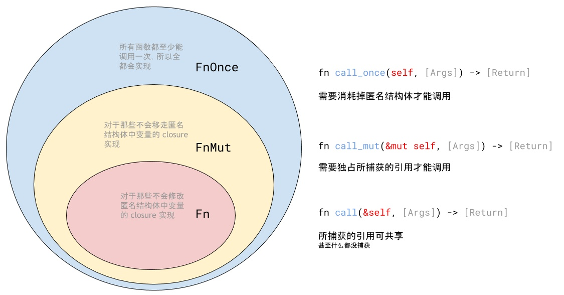
Closure type of rust (difference between FN, fnmut and fnone)
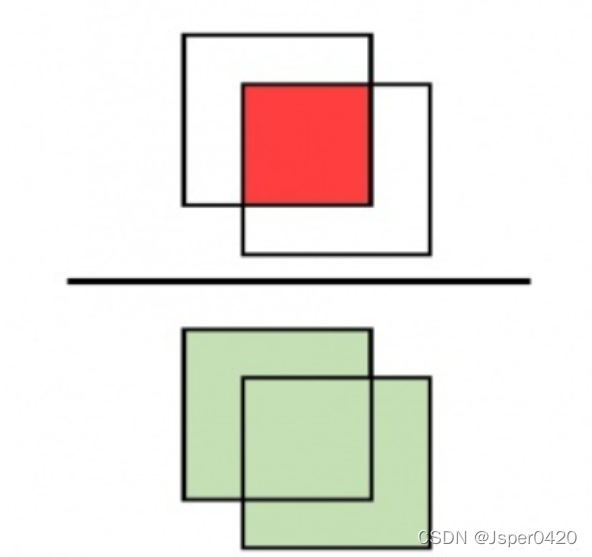
Deep learning classic network analysis and target detection (I): r-cnn
Re expression régulière
MySQL_ 01_ Simple data retrieval
C# 网络相关操作
Clion installation tutorial

Visualization of residential house prices
Jenkspy package installation

随机推荐
The vivado project corresponding to the board is generated by TCL script
JD freefuck Jingdong HaoMao control panel background Command Execution Vulnerability
【ACM】509. Fibonacci number (DP Trilogy)
纳米技术+AI赋能蛋白质组学|珞米生命科技完成近千万美元融资
Crawl lottery data
positioner
解决报错max virtual memory areas vm.max_map_count [65530] is too low, increase to at least [262144]
Crack sliding verification code
Differences between SSD hard disk SATA interface and m.2 interface (detailed summary)
Win1远程出现“这可能是由于credssp加密oracle修正”解决办法
C language to achieve 2048 small game direction merging logic
Nodejs installation
Auto.js 自定义对话框
解决允许在postman中写入注释请求接口方法
powerdesigner各种字体设置;preview字体设置;sql字体设置
Correct opening method of option
Selenium + phantom JS crack sliding verification 2
Excel opens large CSV format data
MATLAB从入门到精通(二)
Software test summary