当前位置:网站首页>Timing model: gated cyclic unit network (Gru)
Timing model: gated cyclic unit network (Gru)
2022-04-23 15:39:00 【HadesZ~】
1. Model definition
Gated loop unit network (Gated Recurrent Unit,GRU)1 Is in LSTM A simplified variant developed on the basis of , It can usually achieve the same speed as LSTM The effect of the model is similar 2.
2. Model structure and forward propagation formula
GRU The hidden state calculation module of the model does not introduce additional memory units , The logic gate is simplified to Reset door (reset gate) and Update door (update gate), Its structural diagram and forward propagation formula are as follows :
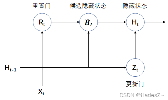
{ transport Enter into : X t ∈ R m × d , H t − 1 ∈ R m × h heavy Set up door : R t = σ ( X t W x r + H t − 1 W h r + b r ) , W x r ∈ R d × h , W h r ∈ R h × h Hou choose implicit hidden shape state : H ~ t = t a n h ( X t W x h + ( R t ⊙ H t − 1 ) W h h + b h ) , W x h ∈ R d × h , W h h ∈ R h × h more new door : Z t = σ ( X t W x z + H t − 1 W h z + b z ) , W x z ∈ R d × h , W h z ∈ R h × h implicit hidden shape state : H t = Z t ⊙ H t − 1 + ( 1 − Z t ) ⊙ H ~ t transport Out : Y ^ t = H t W h y + b y , W h y ∈ R h × q damage loss Letter Count : L = ∑ t = 1 T l ( ( ^ Y ) t , Y t ) (2.1) \begin{cases} Input : & X_t \in R^{m \times d}, \ \ \ \ H_{t-1} \in R^{m \times h} \\ \\ Reset door : & R_t = \sigma(X_tW_{xr} + H_{t-1}W_{hr} + b_r), & W_{xr} \in R^{d \times h},\ \ W_{hr} \in R^{h \times h} \\ \\ Candidate hidden status : & \tilde{H}_t = tanh(X_tW_{xh} + (R_t \odot H_{t-1})W_{hh} + b_h),\ \ & W_{xh} \in R^{d \times h},\ \ W_{hh} \in R^{h \times h} \\ \\ Update door : & Z_t = \sigma(X_tW_{xz} + H_{t-1}W_{hz} + b_z), & W_{xz} \in R^{d \times h},\ \ W_{hz} \in R^{h \times h} \\ \\ Hidden state : & H_t = Z_t \odot H_{t-1} + (1-Z_t) \odot \tilde{H}_t \\ \\ Output : & \hat{Y}_t = H_tW_{hy} + b_y, & W_{hy} \in R^{h \times q} \\ \\ Loss function : & L = \sum_{t=1}^{T} l(\hat(Y)_t, Y_t) \end{cases} \tag{2.1} ⎩⎪⎪⎪⎪⎪⎪⎪⎪⎪⎪⎪⎪⎪⎪⎪⎪⎪⎪⎪⎪⎪⎪⎪⎪⎪⎨⎪⎪⎪⎪⎪⎪⎪⎪⎪⎪⎪⎪⎪⎪⎪⎪⎪⎪⎪⎪⎪⎪⎪⎪⎪⎧ transport Enter into : heavy Set up door : Hou choose implicit hidden shape state : more new door : implicit hidden shape state : transport Out : damage loss Letter Count :Xt∈Rm×d, Ht−1∈Rm×hRt=σ(XtWxr+Ht−1Whr+br),H~t=tanh(XtWxh+(Rt⊙Ht−1)Whh+bh), Zt=σ(XtWxz+Ht−1Whz+bz),Ht=Zt⊙Ht−1+(1−Zt)⊙H~tY^t=HtWhy+by,L=∑t=1Tl((^Y)t,Yt)Wxr∈Rd×h, Whr∈Rh×hWxh∈Rd×h, Whh∈Rh×hWxz∈Rd×h, Whz∈Rh×hWhy∈Rh×q(2.1)
3. GRU Back propagation process
Because no additional memory units are introduced , therefore GRU Back propagation calculation diagram and RNN Agreement ( Such as the author's article : Time series model : Cyclic neural network (RNN) Chinese 3 Shown ),GRU The back propagation formula is as follows :
∂ L ∂ Y ^ t = ∂ l ( Y ^ t , Y t ) T ⋅ ∂ Y ^ t (3.1) \frac{\partial L}{\partial \hat{Y}_t} = \frac{\partial l(\hat{Y}_t, Y_t)}{T \cdot\partial \hat{Y}_t} \tag {3.1} ∂Y^t∂L=T⋅∂Y^t∂l(Y^t,Yt)(3.1)
∂ L ∂ Y ^ t ⇒ { ∂ L ∂ W h y = ∂ L ∂ Y ^ t ∂ Y ^ t ∂ W h y ∂ L ∂ H t = { ∂ L ∂ Y ^ t ∂ Y ^ t ∂ H t , t = T ∂ L ∂ Y ^ t ∂ Y ^ t ∂ H t + ∂ L ∂ H t + 1 ∂ H t + 1 ∂ H t , t < T (3.2) \frac{\partial L}{\partial \hat{Y}_t} \Rightarrow \begin{cases} \frac{\partial L}{\partial W_{hy}} = \frac{\partial L}{\partial \hat{Y}_t} \frac{\partial \hat{Y}_t}{\partial W_{hy}} \\ \\ \frac{\partial L}{\partial H_t} = \begin{cases} \frac{\partial L}{\partial \hat{Y}_t} \frac{\partial \hat{Y}_t}{\partial H_t}, & t=T \\ \\ \frac{\partial L}{\partial \hat{Y}_t} \frac{\partial \hat{Y}_t}{\partial H_t} + \frac{\partial L}{\partial H_{t+1}}\frac{\partial H_{t+1}}{\partial H_{t}}, & t<T \end{cases} \end{cases} \tag {3.2} ∂Y^t∂L⇒⎩⎪⎪⎪⎪⎪⎪⎪⎨⎪⎪⎪⎪⎪⎪⎪⎧∂Why∂L=∂Y^t∂L∂Why∂Y^t∂Ht∂L=⎩⎪⎪⎨⎪⎪⎧∂Y^t∂L∂Ht∂Y^t,∂Y^t∂L∂Ht∂Y^t+∂Ht+1∂L∂Ht∂Ht+1,t=Tt<T(3.2)
{ ∂ L ∂ W x z = ∂ L ∂ Z t ∂ Z t ∂ W x z ∂ L ∂ W h z = ∂ L ∂ Z t ∂ Z t ∂ W h z ∂ L ∂ b z = ∂ L ∂ Z t ∂ Z t ∂ b z { ∂ L ∂ W x h = ∂ L ∂ H ~ t ∂ H ~ t ∂ W x h ∂ L ∂ W h h = ∂ L ∂ H ~ t ∂ H ~ t ∂ W h h ∂ L ∂ b h = ∂ L ∂ H ~ t ∂ H ~ t ∂ b h (3.3) \begin{matrix} \begin{cases} \frac{\partial L}{\partial W_{xz}} = \frac{\partial L}{\partial Z_{t}}\frac{\partial Z_{t}}{\partial W_{xz}} \\ \\ \frac{\partial L}{\partial W_{hz}} = \frac{\partial L}{\partial Z_{t}}\frac{\partial Z_{t}}{\partial W_{hz}} \\ \\ \frac{\partial L}{\partial b_{z}} = \frac{\partial L}{\partial Z_{t}}\frac{\partial Z_{t}}{\partial b_{z}} \end{cases} & & & & \begin{cases} \frac{\partial L}{\partial W_{xh}} = \frac{\partial L}{\partial \tilde{H}_t}\frac{\partial \tilde{H}_t}{\partial W_{xh}} \\ \\ \frac{\partial L}{\partial W_{hh}} = \frac{\partial L}{\partial \tilde{H}_t}\frac{\partial \tilde{H}_t}{\partial W_{hh}} \\ \\ \frac{\partial L}{\partial b_{h}} = \frac{\partial L}{\partial \tilde{H}_t}\frac{\partial \tilde{H}_t}{\partial b_{h}} \end{cases} \end{matrix} \tag {3.3} ⎩⎪⎪⎪⎪⎪⎪⎨⎪⎪⎪⎪⎪⎪⎧∂Wxz∂L=∂Zt∂L∂Wxz∂Zt∂Whz∂L=∂Zt∂L∂Whz∂Zt∂bz∂L=∂Zt∂L∂bz∂Zt⎩⎪⎪⎪⎪⎪⎪⎪⎨⎪⎪⎪⎪⎪⎪⎪⎧∂Wxh∂L=∂H~t∂L∂Wxh∂H~t∂Whh∂L=∂H~t∂L∂Whh∂H~t∂bh∂L=∂H~t∂L∂bh∂H~t(3.3)
{ ∂ L ∂ W x r = ∂ L ∂ R t ∂ R t ∂ W x r ∂ L ∂ W h r = ∂ L ∂ R t ∂ R t ∂ W h r ∂ L ∂ b r = ∂ L ∂ R t ∂ R t ∂ b r (3.4) \begin{cases} \frac{\partial L}{\partial W_{xr}} = \frac{\partial L}{\partial R_{t}}\frac{\partial R_{t}}{\partial W_{xr}} \\ \\ \frac{\partial L}{\partial W_{hr}} = \frac{\partial L}{\partial R_{t}}\frac{\partial R_{t}}{\partial W_{hr}} \\ \\ \frac{\partial L}{\partial b_{r}} = \frac{\partial L}{\partial R_{t}}\frac{\partial R_{t}}{\partial b_{r}} \end{cases} \tag {3.4} ⎩⎪⎪⎪⎪⎪⎪⎨⎪⎪⎪⎪⎪⎪⎧∂Wxr∂L=∂Rt∂L∂Wxr∂Rt∂Whr∂L=∂Rt∂L∂Whr∂Rt∂br∂L=∂Rt∂L∂br∂Rt(3.4)
And LSTM Empathy ,GRU The key to the solution of the back propagation formula is also the calculation of different time steps ( Pass on ) gradient The solution of , The method is similar to LSTM Consistent, this article will not repeat . And we can also draw qualitative conclusions ,GRU Principles and methods of alleviating long-term dependence LSTM similar , It is realized by adjusting the multiplier of high-order power term and adding low-order power term . among , Resetting the gate helps capture short-term dependencies in the sequence , Update gates help capture long-term dependencies in sequences .( Please refer to the author's article for details : Time series model : Long and short term memory network (LSTM) The proof process in )
4. Code implementation of the model
4.1 TensorFlow Framework implementations
4.2 Pytorch Framework implementations
import torch
from torch import nn
from torch.nn import functional as F


#
class Dense(nn.Module):
    """ Args: outputs_dim: Positive integer, dimensionality of the output space. activation: Activation function to use. If you don't specify anything, no activation is applied (ie. "linear" activation: `a(x) = x`). use_bias: Boolean, whether the layer uses a bias vector. kernel_initializer: Initializer for the `kernel` weights matrix. bias_initializer: Initializer for the bias vector. Input shape: N-D tensor with shape: `(batch_size, ..., input_dim)`. The most common situation would be a 2D input with shape `(batch_size, input_dim)`. Output shape: N-D tensor with shape: `(batch_size, ..., units)`. For instance, for a 2D input with shape `(batch_size, input_dim)`, the output would have shape `(batch_size, units)`. """
    def __init__(self, input_dim, output_dim, **kwargs):
        super().__init__()
        #  Hyperparametric definition
        self.use_bias = kwargs.get('use_bias', True)
        self.kernel_initializer = kwargs.get('kernel_initializer', nn.init.xavier_uniform_)
        self.bias_initializer = kwargs.get('bias_initializer', nn.init.zeros_)
        #
        self.Linear = nn.Linear(input_dim, output_dim, bias=self.use_bias)
        self.Activation = kwargs.get('activation', nn.ReLU())
        #  Parameter initialization
        self.kernel_initializer(self.Linear.weight)
        self.bias_initializer(self.Linear.bias)

    def forward(self, inputs):
        outputs = self.Activation(
            self.Linear(inputs)
        )
        return outputs


#
class GRU_Cell(nn.Module):
    def __init__(self, token_dim, hidden_dim
                 , reset_act=nn.ReLU()
                 , update_act=nn.ReLU()
                 , hathid_act=nn.Tanh()
                 , **kwargs):
        super().__init__()
        #
        self.hidden_dim = hidden_dim
        #
        self.ResetG = Dense(
            token_dim + self.hidden_dim, self.hidden_dim
            , activation=reset_act, **kwargs
        )
        self.UpdateG = Dense(
            token_dim + self.hidden_dim, self.hidden_dim
            , activation=update_act, **kwargs
        )
        self.HatHidden = Dense(
            token_dim + self.hidden_dim, self.hidden_dim
            , activation=hathid_act, **kwargs
        )

    def forward(self, inputs, last_state):
        last_hidden = last_state[-1]
        #
        Rg = self.ResetG(
            torch.concat([inputs, last_hidden], dim=1)
        )
        Zg = self.UpdateG(
            torch.concat([inputs, last_hidden], dim=1)
        )
        hat_hidden = self.HatHidden(
            torch.concat([inputs, Rg * last_hidden], dim=1)
        )
        hidden = Zg*last_hidden + (1-Zg)*hat_hidden
        #
        return [hidden]

    def zero_initialization(self, batch_size):
        return torch.zeros([batch_size, self.hidden_dim])


#
class RNN_Layer(nn.Module):
    def __init__(self, rnn_cell, bidirectional=False):
        super().__init__()
        self.RNNCell = rnn_cell
        self.bidirectional = bidirectional

    def forward(self, inputs, mask=None, initial_state=None):
        """ inputs: it's shape is [batch_size, time_steps, token_dim] mask: it's shape is [batch_size, time_steps] :return hidden_state_seqence: its' shape is [batch_size, time_steps, hidden_dim] last_state: it is the hidden state of input sequences at last time step, but, attentively, the last token wouble be a padding token, so this last state is not the real last state of input sequences; if you want to get the real last state of input sequences, please use utils.get_rnn_last_state(hidden_state_seqence). """
        batch_size, time_steps, token_dim = inputs.shape
        #
        if initial_state is None:
            initial_state = self.RNNCell.zero_initialization(batch_size)
        if mask is None:
            if batch_size == 1:
                mask = torch.ones([1, time_steps])
            else:
                raise ValueError(' Please give a mask matrix (mask)')

        #  Forward time step cycle
        hidden_list = []
        hidden_state = initial_state
        for i in range(time_steps):
            hidden_state = self.RNNCell(inputs[:, i], hidden_state)
            hidden_list.append(hidden_state[-1])
            hidden_state = [hidden_state[j] * mask[:, i:i+1] + initial_state[j] * (1-mask[:, i:i+1])
                            for j in range(len(hidden_state))]  #  Reinitialize ( Addend function )
        #
        seqences = torch.reshape(
            torch.unsqueeze(
                torch.concat(hidden_list, dim=1), dim=1
            )
            , [batch_size, time_steps, -1]
        )
        last_state = hidden_list[-1]

        #  Reverse time step cycle
        if self.bidirectional is True:
            hidden_list = []
            hidden_state = initial_state
            for i in range(time_steps, 0, -1):
                hidden_state = self.RNNCell(inputs[:, i-1], hidden_state)
                hidden_list.append(hidden_state[-1])
                hidden_state = [hidden_state[j] * mask[:, i-1:i] + initial_state[j] * (1 - mask[:, i-1:i])
                                for j in range(len(hidden_state))]  #  Reinitialize ( Addend function )
            #
            seqences = torch.concat([
                seqences,
                torch.reshape(
                    torch.unsqueeze(
                        torch.concat(hidden_list, dim=1), dim=1)
                    , [batch_size, time_steps, -1])
                ]
                , dim=-1
            )
            last_state = torch.concat([
                last_state
                , hidden_list[-1]
                ]
                , dim=-1
            )

        return {

            'hidden_state_seqences': seqences
            , 'last_state': last_state
        }
Cho, K., Van Merriënboer, B., Bahdanau, D., & Bengio, Y. (2014). On the properties of neural machine translation: encoder-decoder approaches. arXiv preprint arXiv:1409.1259. ︎
Chung, J., Gulcehre, C., Cho, K., & Bengio, Y. (2014). Empirical evaluation of gated recurrent neural networks on sequence modeling. arXiv preprint arXiv:1412.3555. ︎
版权声明
本文为[HadesZ~]所创,转载请带上原文链接,感谢
https://yzsam.com/2022/04/202204231536010859.html
边栏推荐
- 幂等性的处理
- Crawling fragment of a button style on a website
- Explanation of redis database (IV) master-slave replication, sentinel and cluster
- 【递归之数的拆分】n分k,限定范围的拆分
- 如果conda找不到想要安装的库怎么办PackagesNotFoundError: The following packages are not available from current
- 自主作业智慧农场创新论坛
- G007-HWY-CC-ESTOR-03 华为 Dorado V6 存储仿真器搭建
- cadence SPB17. 4 - Active Class and Subclass
- CAP定理
- 怎么看基金是不是reits,通过银行购买基金安全吗
猜你喜欢
Knn,Kmeans和GMM
网站建设与管理的基本概念

Demonstration meeting on startup and implementation scheme of swarm intelligence autonomous operation smart farm project
What exactly does the distributed core principle analysis that fascinates Alibaba P8? I was surprised after reading it
Advantages, disadvantages and selection of activation function
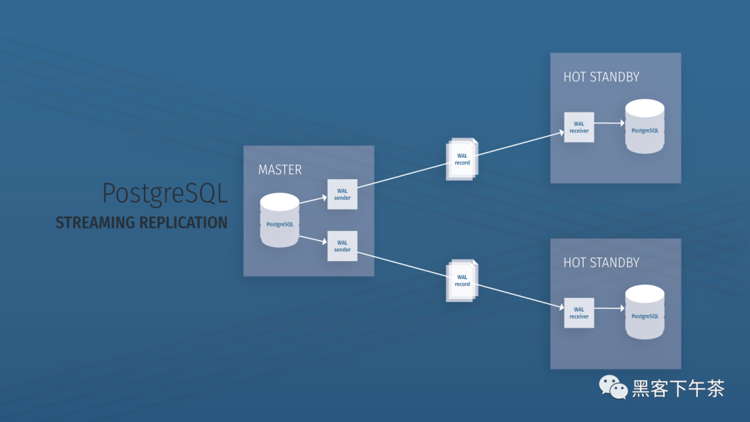
使用 Bitnami PostgreSQL Docker 镜像快速设置流复制集群

Neodynamic Barcode Professional for WPF V11. 0

IronPDF for .NET 2022.4.5455
时序模型:门控循环单元网络(GRU)
Neodynamic Barcode Professional for WPF V11.0
随机推荐
通过 PDO ODBC 将 PHP 连接到 MySQL
Leetcode学习计划之动态规划入门day3(198,213,740)
utils.DeprecatedIn35 因升级可能取消,该如何办
After time judgment of date
Multi level cache usage
Explanation of redis database (I)
Redis主从复制过程
Go语言数组,指针,结构体
自动化测试框架常见类型▏自动化测试就交给软件测评机构
Deep learning - Super parameter setting
网站压测工具Apache-ab,webbench,Apache-Jemeter
网站某个按钮样式爬取片段
现在做自媒体能赚钱吗?看完这篇文章你就明白了
为啥禁用外键约束
木木一路走好呀
PHP classes and objects
What is CNAs certification? What are the software evaluation centers recognized by CNAs?
【递归之数的拆分】n分k,限定范围的拆分
JSON date time date format
Modèle de Cluster MySQL et scénario d'application