当前位置:网站首页>时序模型:长短期记忆网络(LSTM)
时序模型:长短期记忆网络(LSTM)
2022-04-23 15:36:00 【HadesZ~】
1. 模型定义
循环神经网络(RNN)模型存在长期依赖问题,不能有效学习较长时间序列中的特征。长短期记忆网络(long short-term memory,LSTM)1是最早被承认能有效缓解长期依赖问题的改进方案。
2. 模型结构
LSTM的隐藏状态计算模块,在RNN基础上引入一个新的内部状态:记忆细胞(memory cell),和三个控制信息传递的逻辑门:输入门(input gate)、遗忘门(forget gate)、输出门(output gate)。其结构如下图所示:
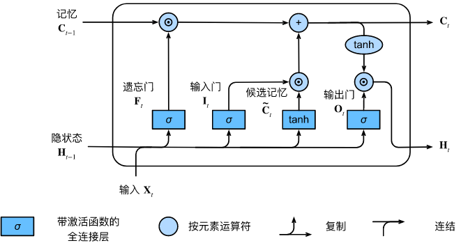
图中,记忆细胞(memory cell)与隐状态具有相同的形状(向量维度),其设计目的是用于记录附加的隐藏状态与输入信息,有些文献认为记忆细胞是一种特殊类型的隐状态;输入门(input gate)控制(本时刻)输入观测和(上时刻)隐藏状态中哪些信息会添加进记忆细胞;遗忘门(forget gate)控制忘记上时刻记忆细胞中的哪些内容;输出门(output gate)控制记忆细胞中哪些信息会输出给隐藏状态。
3. 前向传播
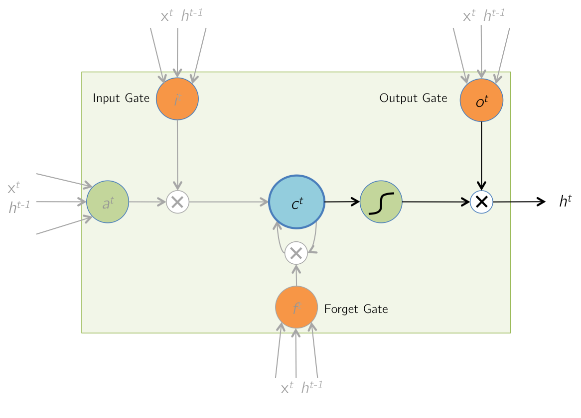
为更容易理解 LSTM 模型的前向传播过程,我们将模型结构图改编为如下所示2(图中 a t a^t at 指 t t t 时刻的候选记忆细胞 C ~ t \tilde{C}_t C~t):
由此我们可以得到 LSTM 模型的前向传播公式:
{ 候 选 记 忆 细 胞 : C ~ t = t a n h ( X t W x c + H t − 1 W h c + b c ) , X t ∈ R m × d , H t − 1 ∈ R m × h , W x c ∈ R d × h , W ∈ R h × h 输 入 门 : I t = σ ( X t W x i + H t − 1 W h i + b i ) , W x i ∈ R d × h , W h i ∈ R h × h 遗 忘 门 : F t = σ ( X t W x f + H t − 1 W h f + b f ) , W x f ∈ R d × h , W h f ∈ R h × h 输 出 门 : O t = σ ( X t W x o + H t − 1 W h o + b o ) , W x o ∈ R d × h , W h o ∈ R h × h (3.1.1) \begin{cases} 候选记忆细胞: & \tilde{C}_t = tanh(X_{t}W_{xc} + H_{t-1}W_{hc} + b_c), & \ \ \ \ X_t \in R^{m \times d}, H_{t-1}\in R^{m \times h}, W_{xc} \in R^{d\times h}, W \in R^{h\times h} \\ \\ 输入门: & I_t = \sigma(X_{t}W_{xi} + H_{t-1}W_{hi} +b_i), & W_{xi} \in R^{d \times h}, W_{hi} \in R^{h \times h} \\ \\ 遗忘门: & F_t = \sigma(X_{t}W_{xf} + H_{t-1}W_{hf} +b_f), & W_{xf} \in R^{d \times h}, W_{hf} \in R^{h \times h} \\ \\ 输出门: & O_t = \sigma(X_{t}W_{xo} + H_{t-1}W_{ho} +b_o), & W_{xo} \in R^{d \times h}, W_{ho} \in R^{h \times h} \end{cases} \tag {3.1.1} ⎩⎪⎪⎪⎪⎪⎪⎪⎪⎪⎪⎨⎪⎪⎪⎪⎪⎪⎪⎪⎪⎪⎧候选记忆细胞:输入门:遗忘门:输出门:C~t=tanh(XtWxc+Ht−1Whc+bc),It=σ(XtWxi+Ht−1Whi+bi),Ft=σ(XtWxf+Ht−1Whf+bf),Ot=σ(XtWxo+Ht−1Who+bo), Xt∈Rm×d,Ht−1∈Rm×h,Wxc∈Rd×h,W∈Rh×hWxi∈Rd×h,Whi∈Rh×hWxf∈Rd×h,Whf∈Rh×hWxo∈Rd×h,Who∈Rh×h(3.1.1)
{ 记 忆 细 胞 : C t = I t ⊙ C ~ t + F t ⊙ C t − 1 隐 藏 状 态 : H t = O t ⊙ t a n h ( C t ) 模 型 输 出 : Y ^ t = H t W h y + b y , W h y ∈ R h × q , Y ^ t ∈ R m × q 损 失 函 数 : L = 1 T ∑ t = 1 T l ( Y ^ t , Y t ) , L ∈ R (3.1.2) \begin{cases} 记忆细胞: & C_t = I_t \odot \tilde{C}_t + F_t \odot C_{t-1} \\ \\ 隐藏状态: & H_t = O_t \odot tanh(C_t) \\ \\ 模型输出: & \hat{Y}_t = H_tW_{hy} + b_y, & W_{hy} \in R^{h \times q}, \ \hat{Y}_t \in R^{m \times q} \\ \\ 损失函数: & L = \frac{1}{T} \sum_{t=1}^{T} l(\hat{Y}_t, Y_t), & L \in R \end{cases} \tag {3.1.2} ⎩⎪⎪⎪⎪⎪⎪⎪⎪⎪⎪⎨⎪⎪⎪⎪⎪⎪⎪⎪⎪⎪⎧记忆细胞:隐藏状态:模型输出:损失函数:Ct=It⊙C~t+Ft⊙Ct−1Ht=Ot⊙tanh(Ct)Y^t=HtWhy+by,L=T1∑t=1Tl(Y^t,Yt),Why∈Rh×q, Y^t∈Rm×qL∈R(3.1.2)
式中 m m m 为小批量随机梯度下降的批量大小(batch size), d d d 为输入单词的词向量维度, h h h、 q q q 为隐藏状态和模型输出的向量宽度(维度)。
4. LSTM缓解长期依赖的原理
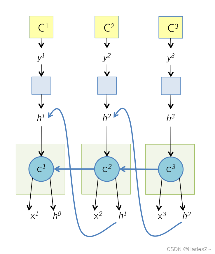
RNN模型存在长期依赖问题,源自于其反向传播过程中存在的梯度消失现象。LSTM模型通过改进RNN模型的梯度传播过程,来缓解反向传播过程中,距离语句结尾处较远的单词容易出现梯度消失的现象。由第3节所述前向传播过程,将LSTM模型反向传播的计算图绘制如下3:
所以根据计算图,可以推导出LSTM模型的反向传播公式为:
∂ L ∂ Y ^ t = ∂ l ( Y ^ t , Y t ) T ⋅ ∂ Y ^ t (4.1) \frac{\partial L}{\partial \hat{Y}_t} = \frac{\partial l(\hat{Y}_t, Y_t)}{T \cdot\partial \hat{Y}_t} \tag {4.1} ∂Y^t∂L=T⋅∂Y^t∂l(Y^t,Yt)(4.1)
∂ L ∂ Y ^ t ⇒ { ∂ L ∂ W h y = ∂ L ∂ Y ^ t ∂ Y ^ t ∂ W h y ∂ L ∂ H t = { ∂ L ∂ Y ^ t ∂ Y ^ t ∂ H t , t = T ∂ L ∂ Y ^ t ∂ Y ^ t ∂ H t + ∂ L ∂ C t + 1 ∂ C t + 1 ∂ H t , t < T (4.2) \frac{\partial L}{\partial \hat{Y}_t} \Rightarrow \begin{cases} \frac{\partial L}{\partial W_{hy}} = \frac{\partial L}{\partial \hat{Y}_t} \frac{\partial \hat{Y}_t}{\partial W_{hy}} \\ \\ \frac{\partial L}{\partial H_t} = \begin{cases} \frac{\partial L}{\partial \hat{Y}_t} \frac{\partial \hat{Y}_t}{\partial H_t}, & t=T \\ \\ \frac{\partial L}{\partial \hat{Y}_t} \frac{\partial \hat{Y}_t}{\partial H_t} + \frac{\partial L}{\partial C_{t+1}}\frac{\partial C_{t+1}}{\partial H_{t}}, & t<T \end{cases} \end{cases} \tag {4.2} ∂Y^t∂L⇒⎩⎪⎪⎪⎪⎪⎪⎪⎨⎪⎪⎪⎪⎪⎪⎪⎧∂Why∂L=∂Y^t∂L∂Why∂Y^t∂Ht∂L=⎩⎪⎪⎨⎪⎪⎧∂Y^t∂L∂Ht∂Y^t,∂Y^t∂L∂Ht∂Y^t+∂Ct+1∂L∂Ht∂Ct+1,t=Tt<T(4.2)
∂ L ∂ H t ⇒ { ∂ L ∂ O t = ∂ L ∂ H t ∂ H t ∂ O t ∂ L ∂ C t = { ∂ L ∂ H t ∂ H t ∂ C t , t = T ∂ L ∂ H t ∂ H t ∂ C t + ∂ L ∂ H t ∂ C t + 1 ∂ C t , t < T (4.3) \frac{\partial L}{\partial H_t} \Rightarrow \begin{cases} \frac{\partial L}{\partial O_t} = \frac{\partial L}{\partial H_t} \frac{\partial H_t}{\partial O_t} \\ \\ \frac{\partial L}{\partial C_t} = \begin{cases} \frac{\partial L}{\partial H_t} \frac{\partial H_t}{\partial C_t}, & t=T \\ \\ \frac{\partial L}{\partial H_t} \frac{\partial H_t}{\partial C_t} + \frac{\partial L}{\partial H_t} \frac{\partial C_{t+1}}{\partial C_{t}}, & t<T \end{cases} \end{cases} \tag {4.3} ∂Ht∂L⇒⎩⎪⎪⎪⎪⎪⎪⎨⎪⎪⎪⎪⎪⎪⎧∂Ot∂L=∂Ht∂L∂Ot∂Ht∂Ct∂L=⎩⎪⎨⎪⎧∂Ht∂L∂Ct∂Ht,∂Ht∂L∂Ct∂Ht+∂Ht∂L∂Ct∂Ct+1,t=Tt<T(4.3)
∂ L ∂ O t ⇒ { ∂ L ∂ W x o = ∂ L ∂ O t ∂ O t ∂ W x o ∂ L ∂ W h o = ∂ L ∂ O t ∂ O t ∂ W h o ∂ L ∂ b o = ∂ L ∂ O t ∂ O t ∂ b o ∂ L ∂ C t ⇒ { ∂ L ∂ C ~ t = ∂ L ∂ C t ∂ C t ∂ C ~ t ∂ L ∂ I t = ∂ L ∂ C t ∂ C t ∂ I t ∂ L ∂ F t = ∂ L ∂ C t ∂ C t ∂ F t (4.4) \begin{matrix} \frac{\partial L}{\partial O_t} \Rightarrow \begin{cases} \frac{\partial L}{\partial W_{xo}} = \frac{\partial L}{\partial O_t} \frac{\partial O_t}{\partial W_{xo}} \\ \\ \frac{\partial L}{\partial W_{ho}} = \frac{\partial L}{\partial O_t} \frac{\partial O_t}{\partial W_{ho}} \\ \\ \frac{\partial L}{\partial b_{o}} = \frac{\partial L}{\partial O_t} \frac{\partial O_t}{\partial b_{o}} \end{cases} & & & \frac{\partial L}{\partial C_t} \Rightarrow \begin{cases} \frac{\partial L}{\partial \tilde{C}_t} = \frac{\partial L}{\partial C_t} \frac{\partial C_t}{\partial \tilde{C}_t} \\\\ \frac{\partial L}{\partial I_t} = \frac{\partial L}{\partial C_t} \frac{\partial C_t}{\partial I_t} \\\\ \frac{\partial L}{\partial F_t} = \frac{\partial L}{\partial C_t} \frac{\partial C_t}{\partial F_t} \end{cases} \end{matrix} \tag {4.4} ∂Ot∂L⇒⎩⎪⎪⎪⎪⎪⎪⎨⎪⎪⎪⎪⎪⎪⎧∂Wxo∂L=∂Ot∂L∂Wxo∂Ot∂Who∂L=∂Ot∂L∂Who∂Ot∂bo∂L=∂Ot∂L∂bo∂Ot∂Ct∂L⇒⎩⎪⎪⎪⎪⎪⎪⎨⎪⎪⎪⎪⎪⎪⎧∂C~t∂L=∂Ct∂L∂C~t∂Ct∂It∂L=∂Ct∂L∂It∂Ct∂Ft∂L=∂Ct∂L∂Ft∂Ct(4.4)
∂ L ∂ C ~ t ⇒ { ∂ L ∂ W x c = ∂ L ∂ C ~ t ∂ C ~ t ∂ W x c ∂ L ∂ W h c = ∂ L ∂ C ~ t ∂ C ~ t ∂ W h c ∂ L ∂ b c = ∂ L ∂ C ~ t ∂ C ~ t ∂ b c ∂ L ∂ I t ⇒ { ∂ L ∂ W x i = ∂ L ∂ I t ∂ I t ∂ W x i ∂ L ∂ W h i = ∂ L ∂ I t ∂ I t ∂ W h i ∂ L ∂ b i = ∂ L ∂ I t ∂ I t ∂ b i ∂ L ∂ F t ⇒ { ∂ L ∂ W x f = ∂ L ∂ F t ∂ F t ∂ W x f ∂ L ∂ W h f = ∂ L ∂ F t ∂ F t ∂ W h f ∂ L ∂ b f = ∂ L ∂ F t ∂ F t ∂ b f (4.5) \begin{matrix} \frac{\partial L}{\partial \tilde{C}_t} \Rightarrow \begin{cases} \frac{\partial L}{\partial W_{xc}} = \frac{\partial L}{\partial \tilde{C}_t} \frac{\partial \tilde{C}_t}{\partial W_{xc}} \\ \\ \frac{\partial L}{\partial W_{hc}} = \frac{\partial L}{\partial \tilde{C}_t} \frac{\partial \tilde{C}_t}{\partial W_{hc}} \\ \\ \frac{\partial L}{\partial b_{c}} = \frac{\partial L}{\partial \tilde{C}_t} \frac{\partial \tilde{C}_t}{\partial b_{c}} \end{cases} & & & \frac{\partial L}{\partial I_t} \Rightarrow \begin{cases} \frac{\partial L}{\partial W_{xi}} = \frac{\partial L}{\partial I_t} \frac{\partial I_t}{\partial W_{xi}} \\ \\ \frac{\partial L}{\partial W_{hi}} = \frac{\partial L}{\partial I_t} \frac{\partial I_t}{\partial W_{hi}} \\ \\ \frac{\partial L}{\partial b_{i}} = \frac{\partial L}{\partial I_t} \frac{\partial I_t}{\partial b_{i}} \end{cases} & & & \frac{\partial L}{\partial F_t} \Rightarrow \begin{cases} \frac{\partial L}{\partial W_{xf}} = \frac{\partial L}{\partial F_t} \frac{\partial F_t}{\partial W_{xf}} \\ \\ \frac{\partial L}{\partial W_{hf}} = \frac{\partial L}{\partial F_t} \frac{\partial F_t}{\partial W_{hf}} \\ \\ \frac{\partial L}{\partial b_{f}} = \frac{\partial L}{\partial F_t} \frac{\partial F_t}{\partial b_{f}} \end{cases} \end{matrix} \tag {4.5} ∂C~t∂L⇒⎩⎪⎪⎪⎪⎪⎪⎪⎨⎪⎪⎪⎪⎪⎪⎪⎧∂Wxc∂L=∂C~t∂L∂Wxc∂C~t∂Whc∂L=∂C~t∂L∂Whc∂C~t∂bc∂L=∂C~t∂L∂bc∂C~t∂It∂L⇒⎩⎪⎪⎪⎪⎪⎪⎨⎪⎪⎪⎪⎪⎪⎧∂Wxi∂L=∂It∂L∂Wxi∂It∂Whi∂L=∂It∂L∂Whi∂It∂bi∂L=∂It∂L∂bi∂It∂Ft∂L⇒⎩⎪⎪⎪⎪⎪⎪⎨⎪⎪⎪⎪⎪⎪⎧∂Wxf∂L=∂Ft∂L∂Wxf∂Ft∂Whf∂L=∂Ft∂L∂Whf∂Ft∂bf∂L=∂Ft∂L∂bf∂Ft(4.5)
可见反向传播公式的难点是对 式 ( 4.2 ) 式(4.2) 式(4.2)和 式 ( 4.3 ) 式(4.3) 式(4.3)中,不同时间步间的(传递)梯度 ∂ C t + 1 / ∂ H t \partial C_{t+1} / \partial H_{t} ∂Ct+1/∂Ht 和 ∂ C t + 1 / ∂ C t \partial C_{t+1} / \partial C_{t} ∂Ct+1/∂Ct 的求解;而其他梯度项求解十分容易,本文便不做过多展开了。
本文自 t = T t=T t=T 时刻,逐(时间)步反向传播推算出每时刻损失函数对模型隐藏状态的偏导数后,根据数学归纳法得到损失函数对模型隐藏状态的梯度公式为(推导过程见作者符号计算程序:LSTM模型缓解长期依赖问题的数学证明(符号计算程序)):
$$
$$
可见,LSTM模型是通过增加模型参数的低阶幂次项和在每个模型参数的幂次项前添加可变(通过模型训练改变)的乘数项,来缓解参数高阶幂次项趋近于0引起的梯度消失问题。
关于参数高阶幂次项引发的梯度消失问题,更详细解释可见作者文章:时序模型:循环神经网络(RNN)中关于式(3.5)和式(3.9)的解释。
5. 模型的代码实现
5.1 TensorFlow 框架实现
5.2 Pytorch 框架实现
import torch
from torch import nn
from torch.nn import functional as F


#
class Dense(nn.Module):
    """ Args: outputs_dim: Positive integer, dimensionality of the output space. activation: Activation function to use. If you don't specify anything, no activation is applied (ie. "linear" activation: `a(x) = x`). use_bias: Boolean, whether the layer uses a bias vector. kernel_initializer: Initializer for the `kernel` weights matrix. bias_initializer: Initializer for the bias vector. Input shape: N-D tensor with shape: `(batch_size, ..., input_dim)`. The most common situation would be a 2D input with shape `(batch_size, input_dim)`. Output shape: N-D tensor with shape: `(batch_size, ..., units)`. For instance, for a 2D input with shape `(batch_size, input_dim)`, the output would have shape `(batch_size, units)`. """
    def __init__(self, input_dim, output_dim, **kwargs):
        super().__init__()
        # 超参定义
        self.use_bias = kwargs.get('use_bias', True)
        self.kernel_initializer = kwargs.get('kernel_initializer', nn.init.xavier_uniform_)
        self.bias_initializer = kwargs.get('bias_initializer', nn.init.zeros_)
        #
        self.Linear = nn.Linear(input_dim, output_dim, bias=self.use_bias)
        self.Activation = kwargs.get('activation', nn.ReLU())
        # 参数初始化
        self.kernel_initializer(self.Linear.weight)
        self.bias_initializer(self.Linear.bias)

    def forward(self, inputs):
        outputs = self.Activation(
            self.Linear(inputs)
        )
        return outputs


#
class LSTM_Cell(nn.Module):
    def __init__(self, token_dim, hidden_dim
                 , input_act=nn.ReLU()
                 , forget_act=nn.ReLU()
                 , output_act=nn.ReLU()
                 , hatcell_act=nn.Tanh()
                 , hidden_act=nn.Tanh()
                 , **kwargs):
        super().__init__()
        #
        self.hidden_dim = hidden_dim
        #
        self.InputG = Dense(
            token_dim + self.hidden_dim, self.hidden_dim
            , activation=input_act, **kwargs
        )
        self.ForgetG = Dense(
            token_dim + self.hidden_dim, self.hidden_dim
            , activation=forget_act, **kwargs
        )
        self.OutputG = Dense(
            token_dim + self.hidden_dim, self.hidden_dim
            , activation=output_act, **kwargs
        )
        self.HatCell = Dense(
            token_dim + self.hidden_dim, self.hidden_dim
            , activation=hatcell_act, **kwargs
        )
        self.HiddenActivation = hidden_act

    def forward(self, inputs, last_state):
        """ inputs: it is the word vector of this time step token. last_state: last_state = [last_cell, last_hidden_state] :return: """
        last_cell, last_hidden = last_state
        #
        Ig = self.InputG(
            torch.concat([inputs, last_hidden], dim=1)
        )
        Fg = self.ForgetG(
            torch.concat([inputs, last_hidden], dim=1)
        )
        Og = self.OutputG(
            torch.concat([inputs, last_hidden], dim=1)
        )
        hat_cell = self.HatCell(
            torch.concat([inputs, last_hidden], dim=1)
        )
        cell = Fg*last_cell + Ig*hat_cell
        hidden = Og * self.HiddenActivation(cell)
        #
        return [cell, hidden]

    def zero_initialization(self, batch_size):
        init_cell = torch.zeros([batch_size, self.hidden_dim])
        init_state = torch.zeros([batch_size, self.hidden_dim])
        return [init_cell, init_state]


#
class RNN_Layer(nn.Module):
    def __init__(self, rnn_cell, bidirectional=False):
        super().__init__()
        self.RNNCell = rnn_cell
        self.bidirectional = bidirectional

    def forward(self, inputs, mask=None, initial_state=None):
        """ inputs: it's shape is [batch_size, time_steps, token_dim] mask: it's shape is [batch_size, time_steps] :return hidden_state_seqence: its' shape is [batch_size, time_steps, hidden_dim] last_state: it is the hidden state of input sequences at last time step, but, attentively, the last token wouble be a padding token, so this last state is not the real last state of input sequences; if you want to get the real last state of input sequences, please use utils.get_rnn_last_state(hidden_state_seqence). """
        batch_size, time_steps, token_dim = inputs.shape
        #
        if initial_state is None:
            initial_state = self.RNNCell.zero_initialization(batch_size)
        if mask is None:
            if batch_size == 1:
                mask = torch.ones([1, time_steps])
            else:
                raise ValueError('请给定掩码矩阵(mask)')

        # 正向时间步循环
        hidden_list = []
        hidden_state = initial_state
        for i in range(time_steps):
            hidden_state = self.RNNCell(inputs[:, i], hidden_state)
            hidden_list.append(hidden_state[-1])
            hidden_state = [hidden_state[j] * mask[:, i:i+1] + initial_state[j] * (1-mask[:, i:i+1])
                            for j in range(len(hidden_state))]  # 重新初始化(加数项作用)
        #
        seqences = torch.reshape(
            torch.unsqueeze(
                torch.concat(hidden_list, dim=1), dim=1
            )
            , [batch_size, time_steps, -1]
        )
        last_state = hidden_list[-1]

        # 反向时间步循环
        if self.bidirectional is True:
            hidden_list = []
            hidden_state = initial_state
            for i in range(time_steps, 0, -1):
                hidden_state = self.RNNCell(inputs[:, i-1], hidden_state)
                hidden_list.append(hidden_state[-1])
                hidden_state = [hidden_state[j] * mask[:, i-1:i] + initial_state[j] * (1 - mask[:, i-1:i])
                                for j in range(len(hidden_state))]  # 重新初始化(加数项作用)
            #
            seqences = torch.concat([
                seqences,
                torch.reshape(
                    torch.unsqueeze(
                        torch.concat(hidden_list, dim=1), dim=1)
                    , [batch_size, time_steps, -1])
                ]
                , dim=-1
            )
            last_state = torch.concat([
                last_state
                , hidden_list[-1]
                ]
                , dim=-1
            )

        return {

            'hidden_state_seqences': seqences
            , 'last_state': last_state
        }
Hochreiter, S., & Schmidhuber, J. (1997). Long short-term memory. Neural computation, 9(8), 1735–1780. ︎
版权声明
本文为[HadesZ~]所创,转载请带上原文链接,感谢
https://blog.csdn.net/xunyishuai5020/article/details/123069411
边栏推荐
- 电脑怎么重装系统后显示器没有信号了
- cadence SPB17.4 - Active Class and Subclass
- 深度学习调参的技巧
- Node.js ODBC连接PostgreSQL
- The El tree implementation only displays a certain level of check boxes and selects radio
- Common interview questions of operating system:
- Introduction to dynamic programming of leetcode learning plan day3 (198213740)
- KNN, kmeans and GMM
- Wechat applet customer service access to send and receive messages
- php函数
猜你喜欢
T2 icloud calendar cannot be synchronized
Kubernetes详解(九)——资源配置清单创建Pod实战

考试考试自用

Mobile finance (for personal use)
My raspberry PI zero 2W toss notes to record some problems and solutions

今日睡眠质量记录76分
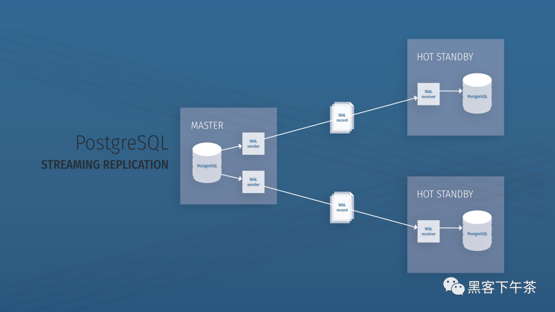
使用 Bitnami PostgreSQL Docker 镜像快速设置流复制集群

Mumu, go all the way
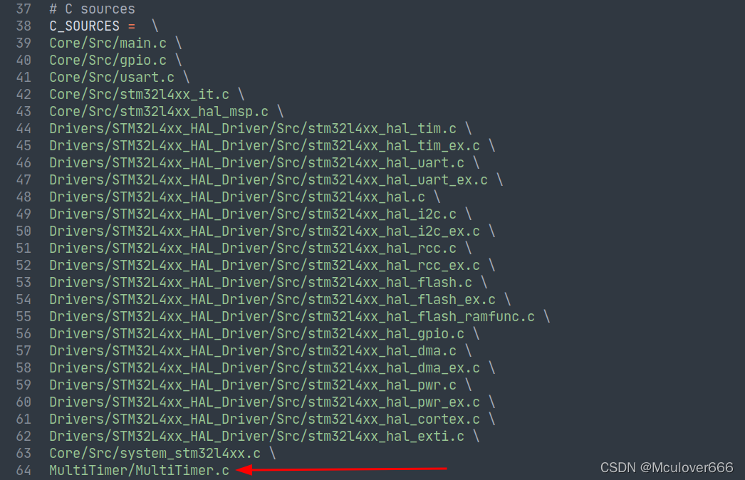
Multitimer V2 reconstruction version | an infinitely scalable software timer

【AI周报】英伟达用AI设计芯片;不完美的Transformer要克服自注意力的理论缺陷
随机推荐
Mumu, go all the way
Node. JS ODBC connection PostgreSQL
Baidu written test 2022.4.12 + programming topic: simple integer problem
Machine learning - logistic regression
Cookie&Session
山寨版归并【上】
c语言---字符串+内存函数
Explanation 2 of redis database (redis high availability, persistence and performance management)
[leetcode daily question] install fence
adobe illustrator 菜单中英文对照
小程序知识点积累
通過 PDO ODBC 將 PHP 連接到 MySQL
fatal error: torch/extension.h: No such file or directory
网站建设与管理的基本概念
G007-HWY-CC-ESTOR-03 华为 Dorado V6 存储仿真器搭建
WPS品牌再升级专注国内,另两款国产软件低调出国门,却遭禁令
ICE -- 源码分析
Special analysis of China's digital technology in 2022
MySQL query library size
HJ31 单词倒排