当前位置:网站首页>Robust Real-time LiDAR-inertial Initialization (Real-time Robust LiDAR Inertial Initialization) Paper Learning
Robust Real-time LiDAR-inertial Initialization (Real-time Robust LiDAR Inertial Initialization) Paper Learning
2022-08-10 03:32:00 【Whiskey Oatmeal Latte】
0 概要
对于大多数的 LiDAR-惯性里程计,Accurate initial condition(包括LiDAR和6轴IMUThe time migration and the transformation between)非常重要,Often seen as advance conditions.但是,The information in their assembly laser radar inertial system may not be able to directly obtain,Often need extra calibration process of space and time ahead,The whole calibration process time-consuming to.
本文提出了LI-Init:A complete and real-time LiDAR-The inertial system initialization process.The process by by LiDAR Measuring estimate the state and IMU Measuring the alignment algorithm based on state,To calibrate the LiDAR 和 IMU 之间的时间偏移、外参、Gravity vector and IMU 偏置.The author will encapsulate the method into the initialization module,To be able to automatically detect the data collected by the movement of the incentive degree.The initialization module can be used in different types of LiDAR-In the inertial combination,And it has been integrated into the most advanced LIO 系统 FAST-LIO2 当中.
本文的具体贡献如下:
- 提出了一种高效、准确、Don't need special time synchronization hardware calibration method to estimate the unknown but constant Lidar-Inertia time migration between,The method based on cross-correlation and unified space-time optimization.
- This paper proposes a new optimization pattern space initialization,And put forward a kind of to evaluate the degree of data movement incentive.Through further by LiDAR Estimate of the state and IMU After noise measurements aligned,The initialization process can automatically extract the initialization required data,And real-time estimation and、重力向量、Gyroscope bias and accelerometer bias.
- In a variety of types of LiDAR-Is carried out on the inertial combination experiment,And verify the efficiency and precision of the initialization process.This method is known the first open source 3 d LiDAR-The inertial system initialization algorithm of time and space,At the same time support the mechanical rotating laser radar and not repeat scanning laser radar.
1 框架概述
整个 LiDAR-The inertial system initialization process framework as shown in the figure below:
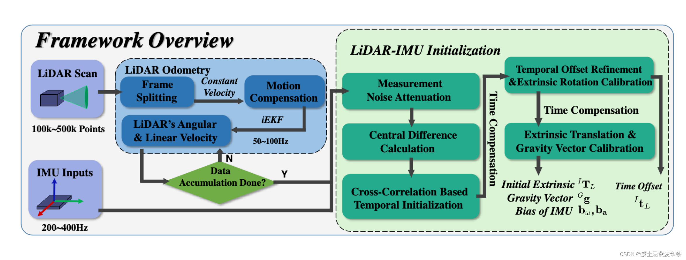
The whole framework consists of two parts:LiDAR 里程计和 LiDAR-Inertial initialization.
1.1 LiDAR 里程计
由于IMUOnly can get incentive in sports,Thus the initialization process is a kind of method based on motion,This means that you need enough exercise motivation.
框架中使用的 LiDAR Odometer is by changing the FAST-LIO2 得到的.LiDAR 里程计在 LiDAR Scanning using uniform model(Includes angular velocity also include linear velocity)来预测 LiDAR Movement and the LiDAR Movement distortion compensation.通过将输入的 LiDAR Frame split into several sub frame,提高 LIDAR Odometer the frame rate of,To relieve the uniform model and the actual movement between the sensor does not match.
如果 LiDAR Odometer no failure(Such as the degradation of),And the estimate of the LiDAR Angular velocity and linear velocity meet the evaluation criteria,Thinks that incentives are sufficient to.这种情况下,就可以将 LiDAR The output of the speedometer and the corresponding IMU The original measurement data to initialize the module.
1.2 LiDAR-Inertial initialization
在初始化过程中,First of all, by moving IMU Measurement data in order to align LiDAR 里程计数据,To calibrate IMU 和 LiDAR Odometer time migration between.The time offset calibration is completed,进行进一步的优化,To further calibration time migration,And calibration parameter、 IMU Bias and gravity vector.
After the initialization of state can be input to tightly coupled LIO 系统中(比如FAST-LIO2),Through the fusion of subsequent LiDAR 数据和 IMU Data for on-line state estimation.
1.3 符号说明
- ⊞ / ⊟ \boxplus/\boxminus ⊞/⊟:On the state of manifold space enclosed“加”和“减”操作
- t k t_{k} tk:第 k k k 次 Lidar Scan the timestamp of the
- ρ j \rho_{j} ρj:一次 Lidar 扫描中的第 j j j A point of time stamp
- τ i \tau_{i} τi:一次 Lidar 扫描中的第 i i i 个 IMU Measuring the timestamp of the
- L j , L k L_{j}, L_{k} Lj,Lk:分别表示 ρ j \rho_{j} ρj 和 t k t_{k} tk 时刻的 Lidar 坐标系
- x , x ^ , x ‾ \mathbf{x}, \widehat{\mathbf{x}}, \overline{\mathbf{x}} x,x,x:Respectively the system state the true value of、Forecast and update the value
- x ~ \widetilde{\mathbf{x}} x:表示真值 x \mathbf{x} x 和估计值 x ‾ \overline{\mathbf{x}} x 之间的误差
- x ˇ j \check{\mathbf{x}}_{j} xˇj:Said at the time of back propagation,与 x k \mathbf{x}_{k} xk The estimate x j \mathbf{x}_{j} xj
- I R L , I p L { }^{I} \mathbf{R}_{L},{ }^{I} \mathbf{p}_{L} IRL,IpL:表示从 LiDAR 到 IMU The outside and the rotation and translation
- I t L { }^{I} t_{L} ItL:表示 LiDAR 和 IMU The total time migration between
- b ω , b a \mathbf{b}_{\boldsymbol{\omega}}, \mathbf{b}_{\mathbf{a}} bω,ba:Said gyroscope and accelerometer bias
- G g { }^{G} \mathbf{g} Gg:Said the gravitational acceleration vector
- I i , I k \mathcal{I}_{i}, \mathcal{I}_{k} Ii,Ik:表示在 τ i \tau_{i} τi 和 t k t_{k} tk Moment in the initialization step IMU 数据序列
- I ‾ k \overline{\mathcal{I}}_{k} Ik:Said after using synchronization time stamp t k t_k tk Compensation after initialization time migrationMU数据序列
- L k \mathcal{L}_{k} Lk:表示在 t k t_{k} tk Moment in the initialization step LiDAR 数据
2 LiDAR 里程计
LiDAR Odometer and built figure part(仅仅使用 LiDAR)Based on uniform model,The model assumes that the angular velocity and linear velocity in the interval ( t k , t k + 1 ) \left(t_{k}, t_{k+1}\right) (tk,tk+1) For const( t k t_k tk 和 t k + 1 t_{k+1} tk+1 分别对应两次 LiDAR The end of the scanning time) ,也就是说:
x k + 1 = x k ⊞ ( Δ t f ( x k , w k ) ) (1) \mathbf{x}_{k+1}=\mathbf{x}_{k} \boxplus\left(\Delta t \mathbf{f}\left(\mathbf{x}_{k}, \mathbf{w}_{k}\right)\right)\tag{1} xk+1=xk⊞(Δtf(xk,wk))(1)
其中, Δ t \Delta t Δt Are two scanning time interval,状态矢量 x \mathbf{x} x,噪声 w \mathbf{w} w And discrete state transfer function f \mathbf{f} f 被定义如下:
x = [ G R L G p L G v L ω L ] , w = [ n v n ω ] , f ( x , w ) = [ ω L G v L n v n ω ] (2) \mathbf{x}=\left[\begin{array}{c}{ }^{G} \mathbf{R}_{L} \\{ }^{G} \mathbf{p}_{L} \\{ }^{G} \mathbf{v}_{L} \\\boldsymbol{\omega}_{L}\end{array}\right], \mathbf{w}=\left[\begin{array}{c}\mathbf{n}_{\mathbf{v}} \\\mathbf{n}_{\boldsymbol{\omega}}\end{array}\right], \mathbf{f}(\mathbf{x}, \mathbf{w})=\left[\begin{array}{c}\boldsymbol{\omega}_{L} \\{ }^{G} \mathbf{v}_{L} \\\mathbf{n}_{\mathbf{v}} \\\mathbf{n}_{\boldsymbol{\omega}}\end{array}\right]\tag{2} x=⎣⎡GRLGpLGvLωL⎦⎤,w=[nvnω],f(x,w)=⎣⎡ωLGvLnvnω⎦⎤(2)
其中, G R L ∈ S O ( 3 ) , G p L { }^{G} \mathbf{R}_{L} \in S O(3),{ }^{G} \mathbf{p}_{L} GRL∈SO(3),GpL 表示 LiDAR 在世界坐标系(也就是第一帧 LiDAR The body coordinate system)下的位姿, G v L { }^{G} \mathbf{v}_{L} GvL 表示 LiDAR In the world coordinate system under linear velocity, ω L \boldsymbol{\omega}_{L} ωL 表示 LiDAR 在 LiDAR Their coordinates the angular velocity of. G v L { }^{G} \mathbf{v}_{L} GvL 和 ω L \boldsymbol{\omega}_{L} ωL Respectively is modeled as a gaussian noise n v \mathbf{n}_{\mathbf{v}} nv 和 n ω \mathbf{n}_{\mathbf{\omega}} nω Drive the random walk process.
在公式(1)中,Using encapsulation on state manifold space“加”和“减”Operation for operation.特别的是,对于公式(2)The state of manifold, ⊞ \boxplus ⊞ And the inverse operation of it ⊟ \boxminus ⊟ Were defined as follows:
[ R a ] ⊞ [ r b ] = [ R E x p ( r ) a + b ] ; [ R 1 a ] ⊟ [ R 2 b ] = [ log ( R 2 T R 1 ) a − b ] \left[\begin{array}{c}\mathbf{R} \\\mathbf{a}\end{array}\right] \boxplus\left[\begin{array}{l}\mathbf{r} \\\mathbf{b}\end{array}\right]=\left[\begin{array}{c}\mathbf{R E x p}(\mathbf{r}) \\\mathbf{a}+\mathbf{b}\end{array}\right] ;\left[\begin{array}{c}\mathbf{R}_{1} \\\mathbf{a}\end{array}\right] \boxminus\left[\begin{array}{c}\mathbf{R}_{2} \\\mathbf{b}\end{array}\right]=\left[\begin{array}{c}\log \left(\mathbf{R}_{2}^{T} \mathbf{R}_{1}\right) \\\mathbf{a}-\mathbf{b}\end{array}\right] [Ra]⊞[rb]=[RExp(r)a+b];[R1a]⊟[R2b]=[log(R2TR1)a−b]
其中, R , R 1 , R 2 ∈ S O ( 3 ) \mathbf{R}, \mathbf{R}_{1}, \mathbf{R}_{2} \in S O(3) R,R1,R2∈SO(3), r , a , b ∈ R n \mathbf{r}, \mathbf{a}, \mathbf{b} \in \mathbb{R}^{n} r,a,b∈Rn, Exp ( ⋅ ) : R 3 ↦ S O ( 3 ) \operatorname{Exp}(\cdot): \mathbb{R}^{3} \mapsto S O(3) Exp(⋅):R3↦SO(3) 表示在 S O ( 3 ) S O(3) SO(3) 上的指数映射, log ( ⋅ ) : S O ( 3 ) ↦ R 3 \log (\cdot) :S O(3) \mapsto \mathbb{R}^{3} log(⋅):SO(3)↦R3 Said the logarithmic mapping.
【注意】这里补充一点, ⊞ \boxplus ⊞ And the inverse operation of it ⊟ \boxminus ⊟ In the original paper is defined as:
⊞ S : S × R n → S ⊟ S : S × S → R n \boxplus_{\mathcal{S}}: \mathcal{S} \times \mathbb{R}^{n} \rightarrow \mathcal{S}\\\boxminus_{\mathcal{S}}: \mathcal{S} \times \mathcal{S} \rightarrow \mathbb{R}^{n} ⊞S:S×Rn→S⊟S:S×S→Rn
They are of practical significance for:
- 运算 y = x ⊞ δ y=x \boxplus \delta y=x⊞δ 表示, 在状态 x x x To add a tiny disturbance δ ∈ R n \delta \in \mathbb{R}^{n} δ∈Rn 得到状态 y y y.
- 相反,运算 δ = y ⊟ x \delta=y \boxminus x δ=y⊟x Sure is added to the state x x x 产生状态 y y y 的扰动 δ ∈ R n \delta \in \mathbb{R}^{n} δ∈Rn.
实际上,The speed of the sensor movement may not be constant.In order to reduce the effect of model error,We will laser radar scanning input is divided into several smaller continuous child frame,Within the scope of each frame of time,Sensor movement with uniform model more consistent.
2.1 Based on the iterative kalman filtering error stateESIKF
基于公式(1)Said in a manifold system,We use iterative kalman filter based on the error state(ESIKF)To estimate the system state.ESIKFThe prediction of forecast steps include state and covariance propagation,表示如下:
x ^ k + 1 = x ‾ k ⊞ ( Δ t f ( x ‾ k , 0 ) ) \widehat{\mathbf{x}}_{k+1}=\overline{\mathbf{x}}_{k} \boxplus \left(\Delta t \mathbf{f}\left(\overline{\mathbf{x}}_{k}, \mathbf{0}\right)\right) xk+1=xk⊞(Δtf(xk,0))
P ^ k + 1 = F x ~ P ‾ k F x ~ T + F w Q F w T \widehat{\mathbf{P}}_{k+1}=\mathbf{F}_{\tilde{\mathbf{x}}} \overline{\mathbf{P}}_{k} \mathbf{F}_{\tilde{\mathbf{x}}}^{T}+\mathbf{F}_{\mathbf{w}} \mathbf{Q} \mathbf{F}_{\mathbf{w}}^{T} Pk+1=Fx~PkFx~T+FwQFwT
其中, P \mathbf{P} P 和 Q \mathbf{Q} Q State estimation and process noise w \mathbf{w} w 的协方差矩阵. F x ~ \mathbf{F}_{\tilde{\mathbf{x}}} Fx~ 和 F w \mathbf{F}_{\mathbf{w}} Fw 分别表示如下:
F x ~ = ∂ ( ( x ‾ k ⊞ x ~ k ) ⊞ ( Δ t f ( x ‾ k ⊞ x ~ k , 0 ) ) ⊟ ( x ‾ k ⊞ Δ t f ( x ‾ k , 0 ) ) ) ∂ x ~ k = [ Exp ( − ω ^ L k Δ t ) 0 3 × 3 0 3 × 3 I 3 × 3 Δ t 0 3 × 3 I 3 × 3 I 3 × 3 Δ t 0 3 × 3 0 3 × 3 0 3 × 3 I 3 × 3 0 3 × 3 0 3 × 3 0 3 × 3 0 3 × 3 I 3 × 3 ] \begin{aligned}\mathbf{F}_{\tilde{\mathbf{x}}} &=\frac{\partial\left(\left(\overline{\mathbf{x}}_{k} \boxplus \tilde{\mathbf{x}}_{k}\right) \boxplus\left(\Delta t \mathbf{f}\left(\overline{\mathbf{x}}_{k} \boxplus \tilde{\mathbf{x}}_{k}, \mathbf{0}\right)\right) \boxminus\left(\overline{\mathbf{x}}_{k} \boxplus \Delta t \mathbf{f}\left(\overline{\mathbf{x}}_{k}, \mathbf{0}\right)\right)\right)}{\partial \tilde{\mathbf{x}}_{k}} \\&=\left[\begin{array}{cccc}\operatorname{Exp}\left(-\widehat{\boldsymbol{\omega}}_{L_{k}} \Delta t\right) & \mathbf{0}_{3 \times 3} & \mathbf{0}_{3 \times 3} & \mathbf{I}_{3 \times 3} \Delta t \\\mathbf{0}_{3 \times 3} & \mathbf{I}_{3 \times 3} & \mathbf{I}_{3 \times 3} \Delta t & \mathbf{0}_{3 \times 3} \\\mathbf{0}_{3 \times 3} & \mathbf{0}_{3 \times 3} & \mathbf{I}_{3 \times 3} & \mathbf{0}_{3 \times 3} \\\mathbf{0}_{3 \times 3} & \mathbf{0}_{3 \times 3} & \mathbf{0}_{3 \times 3} & \mathbf{I}_{3 \times 3}\end{array}\right]\end{aligned} Fx~=∂x~k∂((xk⊞x~k)⊞(Δtf(xk⊞x~k,0))⊟(xk⊞Δtf(xk,0)))=⎣⎡Exp(−ωLkΔt)03×303×303×303×3I3×303×303×303×3I3×3ΔtI3×303×3I3×3Δt03×303×3I3×3⎦⎤
F w = ∂ ( x ‾ k ⊞ ( Δ t f ( x ‾ k , w k ) ) ⊟ ( x ‾ k ⊞ Δ t f ( x ‾ k , 0 ) ) ) ∂ w k = [ 0 3 × 3 0 3 × 3 0 3 × 3 0 3 × 3 I 3 × 3 Δ t 0 3 × 3 0 3 × 3 I 3 × 3 Δ t ] (5) \begin{aligned}\mathbf{F}_{\mathbf{w}} &=\frac{\partial\left(\overline{\mathbf{x}}_{k} \boxplus\left(\Delta t \mathbf{f}\left(\overline{\mathbf{x}}_{k}, \mathbf{w}_{k}\right)\right) \boxminus\left(\overline{\mathbf{x}}_{k} \boxplus \Delta t \mathbf{f}\left(\overline{\mathbf{x}}_{k}, \mathbf{0}\right)\right)\right)}{\partial \mathbf{w}_{k}} \\&=\left[\begin{array}{cc}\mathbf{0}_{3 \times 3} & \mathbf{0}_{3 \times 3} \\\mathbf{0}_{3 \times 3} & \mathbf{0}_{3 \times 3} \\\mathbf{I}_{3 \times 3} \Delta t & \mathbf{0}_{3 \times 3} \\\mathbf{0}_{3 \times 3} & \mathbf{I}_{3 \times 3} \Delta t\end{array}\right]\end{aligned}\tag{5} Fw=∂wk∂(xk⊞(Δtf(xk,wk))⊟(xk⊞Δtf(xk,0)))=⎣⎡03×303×3I3×3Δt03×303×303×303×3I3×3Δt⎦⎤(5)
其中, x ~ \tilde{\mathbf{x}} x~ Said error state.
2.2 LiDAR 运动补偿
在我们考虑的问题中,IMU 数据和 LIDAR The data is out of sync,因此采用 IMU Auxiliary motion compensation method is not feasible.
Upon receiving the timestamp t k + 1 t_{k+1} tk+1 The new laser radar scanning after,To compensate for movement distortion,我们将在时间点 ρ j ∈ ( t k , t k + 1 ) \rho_{j} \in\left(t_{k}, t_{k+1}\right) ρj∈(tk,tk+1) Sampling of each point L j p j { }^{L_{j}} \mathbf{p}_{j} Ljpj 投影到 LiDAR 扫描帧 L k + 1 L_{k+1} Lk+1 的最后时刻 t k + 1 t_{k+1} tk+1.Due to the uniform model,我们有: G v ^ L k + 1 = G v ‾ L k , ω ^ L k + 1 = ω ‾ L k { }^{G} \widehat{\mathbf{v}}_{L_{k+1}}={ }^{G} \overline{\mathbf{v}}_{L_{k}}, \widehat{\boldsymbol{\omega}}_{L_{k+1}}=\overline{\boldsymbol{\omega}}_{L_{k}} GvLk+1=GvLk,ωLk+1=ωLk,That is to say, from the point in time ρ i \rho_i ρi 到时间点 t k + 1 t_{k+1} tk+1,Each point cloud of relative transformation as: L k + 1 T L j = ( L k + 1 R ˇ L j , L k + 1 p ˇ L j ) L_{k+1} \mathbf{\mathbf { T }}_{L_{j}}=\left({ }^{L_{k+1}} \check{\mathbf{R}}_{L_{j}},{ }^{L_{k+1}} \check{\mathbf{p}}_{L_{j}}\right) Lk+1TLj=(Lk+1RˇLj,Lk+1pˇLj),其中:
L k + 1 R ˇ L j = Exp ( − ω ^ L k + 1 Δ t j ) L k + 1 p ˇ L j = − G R ^ L k + 1 T G v ^ L k + 1 Δ t j Δ t j = t k + 1 − ρ j (6) \begin{aligned}{}^{L_{k+1}} \check{\mathbf{R}}_{L_{j}} &=\operatorname{Exp}\left(-\widehat{\boldsymbol{\omega}}_{L_{k+1}} \Delta t_{j}\right) \\{}^{L_{k+1}} \check{\mathbf{p}}_{L_{j}} &=-{ }^{G} \widehat{\mathbf{R}}_{L_{k+1}} ^{T} {}^G \widehat{\mathbf{v}}_{L_{k+1}} \Delta t_{j} \\\Delta t_{j} &=t_{k+1}-\rho_{j}\end{aligned}\tag{6} Lk+1RˇLjLk+1pˇLjΔtj=Exp(−ωLk+1Δtj)=−GRLk+1TGvLk+1Δtj=tk+1−ρj(6)
然后,Local measurement points can be L j p j { }^{L_{j}} \mathbf{p}_{j} Ljpj Can be projected to LiDAR 扫描帧 L k + 1 L_{k+1} Lk+1 的最后时刻 t k + 1 t_{k+1} tk+1,也就是:
L k + 1 p j = L k + 1 T ˇ L j L j p j (7) { }^{L_{k+1}} \mathbf{p}_{j}={}^{L_{k+1}} \check{\mathbf{T}}_{L_{j}}{ }^{L_{j}} \mathbf{p}_{j}\tag{7} Lk+1pj=Lk+1TˇLjLjpj(7)
然后,Distortion compensation after scanning { L k + 1 p j } \left\{ {}^{L_{k+1}} \mathbf{p}_{j}\right\} { Lk+1pj} Provides a about an unknown state G T L k + 1 { }^{G} \mathbf{T}_{L_{k+1}} GTLk+1 The implicit measure,Residual said to point to the distance.在此基础上,In the frame of the iterative kalman filtering iterative estimates the state x k + 1 \mathbf{x}_{k+1} xk+1,直到收敛.After convergence of state estimation is expressed as x ‾ k + 1 \overline{\mathbf{x}}_{k+1} xk+1,And then will be used to spread the subsequent IMU 测量.
3 LiDAR-Inertial initialization
上面的 LiDAR The end of the odometer in each scan,即 t k t_k tk 时刻,输出 LiDAR 的角速度 ω L k \boldsymbol{\omega}_{L_{k}} ωLk 和线速度 G v L k { }^{G} \mathbf{v}_{L_{k}} GvLk.同时,IMUBring also for the original measurements,With a timestamp τ i \tau_{i} τi 的角速度 ω m i \omega_{m_{i}} ωmi And linear acceleration a m i \mathbf{a}_{m_{i}} ami.These data are accumulated,And through the incentive criterion to be accessed repeatedly.Once the data collect enough incentive,Is called initialization module,The final output module time migration I t L ∈ R { }^{I} t_{L} \in \mathbb{R} ItL∈R ,外参 I T L = ( I R L , I p L ) ∈ S E ( 3 ) { }^{I} \mathbf{T}_{L}=\left({ }^{I} \mathbf{R}_{L},{ }^{I} \mathbf{p}_{L}\right) \in SE(3) ITL=(IRL,IpL)∈SE(3) ,IMU 偏置 b ω , b a ∈ R 3 \mathbf{b}_{\omega}, \mathbf{b}_{\mathbf{a}} \in \mathbb{R}^{3} bω,ba∈R3 和 G g ∈ R 3 { }^{G} \mathbf{g} \in \mathbb{R}^{3} Gg∈R3.
3.1 数据预处理
IMUOriginal measurements by noise n ω i \mathbf{n}_{\omega_{i}} nωi 和 n a i \mathbf{n}_{\mathbf{a}_{i}} nai 的影响.IMUMeasurement model for:
ω m i = ω i g t + b ω + n ω i , a m i = a i g t + b a + n a i (8) \boldsymbol{\omega}_{m_{i}}=\boldsymbol{\omega}_{i}^{\mathrm{gt}}+\mathbf{b}_{\omega}+\mathbf{n}_{\omega_{i}}, \mathbf{a}_{m_{i}}=\mathbf{a}_{i}^{\mathrm{gt}}+\mathbf{b}_{\mathbf{a}}+\mathbf{n}_{\mathbf{a}_{i}}\tag{8} ωmi=ωigt+bω+nωi,ami=aigt+ba+nai(8)
其中, ω i g t \boldsymbol{\omega}_{i}^{\mathrm{gt}} ωigt 和 a i g t \mathbf{a}_{i}^{\mathrm{gt}} aigt 是IMUThe true value of angular velocity and linear acceleration.同样,来自 LiDAR Odometer estimate ω L k \boldsymbol{\omega}_{L_{k}} ωLk 和 G v L k { }^{G} \mathbf{v}_{L_{k}} GvLk 也包含噪声.
In order to reduce the impact of these high frequency noise,Usually use a**The zero phase low pass filter(a non-causal zero phase low-pass filter)**To filter the noise,Without introducing any filtering delay.Zero phase filter is through backward and run backButterworthLow pass filter to realize,To produce the attenuation of noiseIMU测量 ω I i = ω i g t + b ω , a I i = a i g t + b a \boldsymbol{\omega}_{I_{i}}=\boldsymbol{\omega}_{i}^{\mathrm{gt}}+\mathbf{b}_{\omega}, \mathbf{a}_{I_{i}}=\mathbf{a}_{i}^{\mathrm{gt}}+\mathbf{b}_{\mathbf{a}} ωIi=ωigt+bω,aIi=aigt+ba.为了简洁,Noise attenuation LiDAR Estimates are still expressed as ω L k \boldsymbol{\omega}_{L_{k}} ωLk 和 G v L k { }^{G} \mathbf{v}_{L_{k}} GvLk .
从 LiDAR Odometer estimate ω L k \boldsymbol{\omega}_{L_{k}} ωLk 和 G v L k { }^{G} \mathbf{v}_{L_{k}} GvLk 中,We through the causal central difference(non-causal central difference)的方法可以得到 LiDAR The angular acceleration and linear acceleration Ω L k , G a L k \boldsymbol{\Omega}_{L_{k}},{ }^{G} \mathbf{a}_{L_{k}} ΩLk,GaLk .
最终的 LiDAR Odometer data can be expressed in a collection:
L k = { ω L k , G v L k , Ω L k , G a L k } (9) \mathcal{L}_{k}=\left\{\boldsymbol{\omega}_{L_{k}},{ }^{G} \mathbf{v}_{L_{k}}, \boldsymbol{\Omega}_{L_{k}},{ }^{G} \mathbf{a}_{L_{k}}\right\}\tag{9} Lk={ ωLk,GvLk,ΩLk,GaLk}(9)
类似的,We from the noise attenuation of gyroscope measure ω I i \boldsymbol{\omega}_{I_{i}} ωIi 可以得到 IMU 的角加速度 Ω I i \boldsymbol{\Omega}_{I_{i}} ΩIi,也可以用集合表示:
I i = { ω I i , a I i , Ω I i } (10) \mathcal{I}_{i}=\left\{\boldsymbol{\omega}_{I_{i}}, \mathbf{a}_{I_{i}}, \boldsymbol{\Omega}_{I_{i}}\right\}\tag{10} Ii={ ωIi,aIi,ΩIi}(10)
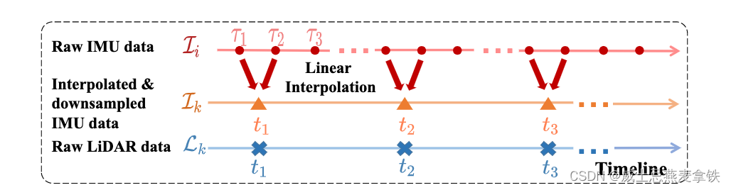
由于 IMU The frequency is generally higher than LiDAR 的频率,Therefore two sequences I i \mathcal{I}_{i} Ii 和 L k \mathcal{L}_{k} Lk 的大小不相同.为了解决此问题,We extracted at the same time LIDAR 和 IMU 数据,And through in everyLiDAR Odometer moment t k t_k tk On linear interpolation for the sampling(如上图).下采样的 IMU 数据表示为 I k \mathcal{I}_{k} Ik:
I k = { ω I k , a I k , Ω I k } (11) \mathcal{I}_{k}=\left\{\boldsymbol{\omega}_{I_{k}}, \mathbf{a}_{I_{k}}, \boldsymbol{\Omega}_{I_{k}}\right\}\tag{11} Ik={ ωIk,aIk,ΩIk}(11)
其具有与 L k \mathcal{L}_{k} Lk 相同的时间戳 t k t_k tk (But the data is actually delayed the time constant of the known I t L { }^{I} t_{L} ItL).
3.2 Through each other(Cross-Correlation)Initialization of time
在大多数情况下,由于 LIDAR-惯性 Odometer module before receiving inevitably, transmission and processing delay,这是LIDAR L k \mathcal{L}_{k} Lk 和IMU I k \mathcal{I}_{k} Ik Between the unknown but constant offset I t L { }^{I} t_{L} ItL,因此如果将 IMU 测量 I k \mathcal{I}_{k} Ik 提前 I t L { }^{I} t_{L} ItL,将与 LIDAR 里程计 L k \mathcal{L}_{k} Lk 对齐.由于 LIDAR 数据和 IMU The data in the discrete time t k t_k tk 中,因此将 IMU Data operation is basically in discrete step size in advance d = I t L / Δ t d = {}^{I}{t_{L}} / \Delta t d=ItL/Δt 中进行的,其中 Δ t \Delta t Δt 是两次 LiDAR Scanning the time interval between.具体而言,For the angular velocity,我们有:
ω I k + d = I R L ω L k + b ω (12) \boldsymbol{\omega}_{I_{k+d}}={ }^{I} \mathbf{R}_{L} \boldsymbol{\omega}_{L_{k}}+\mathbf{b}_{\omega}\tag{12} ωIk+d=IRLωLk+bω(12)
Because of the gyroscope bias b ω \mathbf{b}_{\omega} bω 通常很小,我们可以忽略不计.如果不管 R L \mathbf{R}_{L} RL ,我们发现 ω I k + d \boldsymbol{\omega}_{I_{k+d}} ωIk+d 和 ω L k \boldsymbol{\omega}_{L_{k}} ωLk The size should be the same.We use the similarity between the cross-correlation to quantify the amount of.然后,Can by solving the following optimization problem d d d :
d ∗ = arg max d ∑ ∥ ω I k + d ∥ ⋅ ∥ ω L k ∥ (13) d^{*}=\underset{d}{\arg \max } \sum\left\|\boldsymbol{\omega}_{I_{k+d}}\right\| \cdot\left\|\boldsymbol{\omega}_{L_{k}}\right\|\tag{13} d∗=dargmax∑∥ωIk+d∥⋅∥ωLk∥(13)
即通过在 L k \mathcal{L}_{k} Lk Enumeration migration within the limits of index d d d.
3.3 Unified and the rotation of the parts and time calibration
Cross-correlation method of noise and small scale of gyroscope bias is ruban.但是(13)An obvious defect is time offset calibration resolution than LiDAR A sampling interval odometer Δ t \Delta t Δt ,Therefore cannot identify any less than Δ t \Delta t Δt The deviation of residual δ t \delta t δt.设 I t L { }^{I} t_{L} ItL 为 LiDAR 里程计 ω L \boldsymbol{\omega}_{L} ωL 和 IMU 数据 ω I \boldsymbol{\omega}_{I} ωI The total offset between,则有: I t L = d ∗ Δ t + δ t { }^{I} t_{L}=d^{*} \Delta t+\delta t ItL=d∗Δt+δt.那么将 IMU 测量 ω I \boldsymbol{\omega}_{I} ωI 前移 I t L { }^{I} t_{L} ItL 与 LiDAR 里程计 ω L \boldsymbol{\omega}_{L} ωL 对齐,则公式(12)可以写成:
ω I ( t + I t L ) = I R L ω L ( t ) + b ω (14) \boldsymbol{\omega}_{I}\left(t+{ }^{I} t_{L}\right)={ }^{I} \mathbf{R}_{L} \boldsymbol{\omega}_{L}(t)+\mathbf{b}_{\omega}\tag{14} ωI(t+ItL)=IRLωL(t)+bω(14)
由于在公式(9)中, LiDAR 里程计 ω L \boldsymbol{\omega}_{L} ωL 的数据在 t k t_k tk 时刻得到,将 t = t k t=t_{k} t=tk 和 I t L = d ∗ Δ t + δ t { }^{I} t_{L}=d^{*} \Delta t+\delta t ItL=d∗Δt+δt 代入到公式(14)中有:
ω I ( t k + d ∗ Δ t + δ t ) = I R L ω L k + b ω (15) \boldsymbol{\omega}_{I}\left(t_{k}+d^{*} \Delta t+\delta t\right)={ }^{I} \mathbf{R}_{L} \boldsymbol{\omega}_{L_{k}}+\mathbf{b}_{\omega}\tag{15} ωI(tk+d∗Δt+δt)=IRLωLk+bω(15)
注意到 ω I ( t k + d ∗ Δ t + δ t ) \omega_{I}\left(t_{k}+d^{*} \Delta t+\delta t\right) ωI(tk+d∗Δt+δt) 是 IMU 在时间 t k + d ∗ Δ t t_{k}+d^{*} \Delta t tk+d∗Δt After the angular velocity of,其中在 t k + d ∗ Δ t t_{k}+d^{*} \Delta t tk+d∗Δt 时刻的IMU The angular velocity and angular acceleration respectively: ω I ( t k + d ∗ Δ t ) = ω I k ′ \boldsymbol{\omega}_{I}\left(t_{k}+d^{*} \Delta t\right)=\boldsymbol{\omega}_{I_{k^{\prime}}} ωI(tk+d∗Δt)=ωIk′ 和 Ω I ( t k + d ∗ Δ t ) = Ω I k ′ \boldsymbol{\Omega}_{I}\left(t_{k}+d^{*} \Delta t\right)=\boldsymbol{\Omega}_{I_{k^{\prime}}} ΩI(tk+d∗Δt)=ΩIk′ ( k ′ = k + d ∗ k^{\prime}=k+d^{*} k′=k+d∗ .
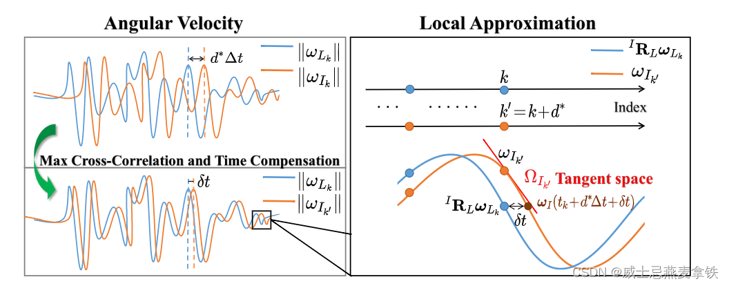
如上图所示,We can, we assume that the δ t \delta t δt This a very small period of time inside the acceleration is constant interpolation to get ω I ( t k + d ∗ Δ t + δ t ) \omega_{I}\left(t_{k}+d^{*} \Delta t+\delta t\right) ωI(tk+d∗Δt+δt),即:
ω I ( t k + d ∗ Δ t + δ t ) ≈ ω I k ′ + δ t Ω I k ′ (16) \boldsymbol{\omega}_{I}\left(t_{k}+d^{*} \Delta t+\delta t\right) \approx \boldsymbol{\omega}_{I_{k^{\prime}}}+\delta t \boldsymbol{\Omega}_{I_{k^{\prime}}}\tag{16} ωI(tk+d∗Δt+δt)≈ωIk′+δtΩIk′(16)
将公式(16)代入到(15)中可以得到:
ω I k ′ + δ t Ω I k ′ = I R L ω L k + b ω (17) \boldsymbol{\omega}_{I_{k^{\prime}}}+\delta t \boldsymbol{\Omega}_{I_{k^{\prime}}}={ }^{I} \mathbf{R}_{L} \boldsymbol{\omega}_{L_{k}}+\mathbf{b}_{\omega}\tag{17} ωIk′+δtΩIk′=IRLωLk+bω(17)
最后,基于(17)中的约束,Unified the optimization problem of space and time can be expressed as:
arg min I R L , b ω , δ t ∑ ∥ I R L ω L k + b ω − ω I k ′ − δ t ⋅ Ω I k ′ ∥ 2 (18) \underset{ { }^{I} \mathbf{R}_{L}, \mathbf{b}_{\omega}, \delta t}{\arg \min } \sum\left\|^{I} \mathbf{R}_{L} \boldsymbol{\omega}_{L_{k}}+\mathbf{b}_{\boldsymbol{\omega}}-\boldsymbol{\omega}_{I_{k^{\prime}}}-\delta t \cdot \boldsymbol{\Omega}_{I_{k^{\prime}}}\right\|^{2}\tag{18} IRL,bω,δtargmin∑∥∥IRLωLk+bω−ωIk′−δt⋅ΩIk′∥∥2(18)
由于存在约束 I R L ∈ S O ( 3 ) { }^{I} \mathbf{R}_{L} \in S O(3) IRL∈SO(3),该问题可以通过 Ceres Solver 进行迭代求解,初值设置为 ( I R L , b ω , δ t ) = ( I 3 × 3 , 0 3 × 1 , 0 ) \left({ }^{I} \mathbf{R}_{L}, \mathbf{b}_{\omega}, \delta t\right)=\left(\mathbf{I}_{3 \times 3}, \mathbf{0}_{3 \times 1}, 0\right) (IRL,bω,δt)=(I3×3,03×1,0).
3.4 Outside and the translation part of the initialization and gravity
在上一节中,We get out and the rotation of the part R L \mathbf{R}_{L} RL,陀螺仪偏置 b ω \mathbf{b}_{\omega} bω 和时间偏移 I t L { }^{I} t_{L} ItL .在本节中,We fixed the values,Then carries on the outside and the translation part of the、The gravity vector and acceleration bias calibration.
首先,We use the good time migration before calibration d ∗ d^{*} d∗ And offset residual δ t \delta t δt 将 IMU 数据 I k \mathcal{I}_{k} Ik 与 LIDAR 的数据 L k \mathcal{L}_{k} Lk 对齐.对齐的IMU数据表示为 I ‾ k \overline{\mathcal{I}}_{k} Ik,Now assume it and L k \mathcal{L}_{k} Lk Completely aligned and have no time to offset.于是,对应于 t k t_k tk 时刻 LiDAR 角速度 ω L k \boldsymbol{\omega}_{L_k} ωLk 的 IMU 角速度 ω ˉ I k \bar{\boldsymbol{\omega}}_{I_{k}} ωˉIk 可以记为:
ω ‾ I k = ω I ( t k + d ∗ Δ t + δ t ) ≈ ω I k + d + δ t Ω I k + d \overline{\boldsymbol{\omega}}_{I_{k}}=\boldsymbol{\omega}_{I}\left(t_{k}+d^{*} \Delta t+\delta t\right) \approx \boldsymbol{\omega}_{I_{k+d}}+\delta t \boldsymbol{\Omega}_{I_{k+d}} ωIk=ωI(tk+d∗Δt+δt)≈ωIk+d+δtΩIk+d
类似的,对应于 t k t_k tk 时刻 LiDAR 线加速度 G a L k { }^{G} \mathbf{a}_{L_{k}} GaLk 的 IMU 线加速度 a ‾ I k \overline{\boldsymbol{a}}_{I_{k}} aIk 可以记为:
a ‾ I k = a I ( t k + d ∗ Δ t + δ t ) ≈ a I k + d + δ t Δ t ( a I k + d + 1 − a I k + d ) \begin{aligned}\overline{\mathbf{a}}_{I_{k}} &=\mathbf{a}_{I}\left(t_{k}+d^{*} \Delta t+\delta t\right) \\& \approx \mathbf{a}_{I_{k+d}}+\frac{\delta t}{\Delta t}\left(\mathbf{a}_{I_{k+d+1}}-\mathbf{a}_{I_{k+d}}\right)\end{aligned} aIk=aI(tk+d∗Δt+δt)≈aIk+d+Δtδt(aIk+d+1−aIk+d)
然后,类似于(14),我们可以找到 IMU 和 LiDAR The acceleration constraints between.在论文中提到,Two outside the fixed reference coordinate system A 和 B Has the following relationship between the acceleration:
A R B a B = a A + ⌊ ω A ⌋ ∧ 2 A p B + ⌊ Ω A ⌋ ∧ A p B { }^{A} \mathbf{R}_{B} \mathbf{a}_{B}=\mathbf{a}_{A}+\left\lfloor\boldsymbol{\omega}_{A}\right\rfloor_{\wedge}^{2} {}^A \mathbf{p}_{B}+\left\lfloor\boldsymbol{\Omega}_{A}\right\rfloor{ }_{\wedge}{ }^{A} \mathbf{p}_{B} ARBaB=aA+⌊ωA⌋∧2ApB+⌊ΩA⌋∧ApB
其中, A R B , A p B { }^{A} \mathbf{R}_{B},{ }^{A} \mathbf{p}_{B} ARB,ApB Says from the coordinate system B 到坐标系 A The outside and transformation of the. a A \mathbf{a}_{A} aA 和 a B \mathbf{a}_{B} aB Are their own coordinates acceleration.
对于 LiDAR-惯性系统,我们有两种选择:用坐标系 A 表示 IMU 坐标系,用坐标系 B 表示 LIDAR 坐标系;或者相反.Notice in the former case, ω A = ω ‾ I k − b ω \boldsymbol{\omega}_{A}=\overline{\boldsymbol{\omega}}_{I_{k}}-\mathbf{b}_{\omega} ωA=ωIk−bω The influence of the accuracy of the gyroscope bias estimation,And angular velocity measurement noise can enlarge Ω A \boldsymbol{\Omega}_{A} ΩA 的误差.In order to avoid this problem and improve upon the translation part of the robustness of calibration,我们将 LIDAR Coordinate system is set to the A,将 IMU 坐标系设置为 坐标系 B.由于 LIDAR 的加速度 G a L k { }^{G} \mathbf{a}_{L_{k}} GaLk Is in the world coordinate system for said,我们需要计算 LiDAR Instant acceleration in LiDAR 坐标系中的表示,记为 a L k \mathbf{a}_{L_{k}} aLk:
a L k = G R L T ( G a L k − G g ) \mathbf{a}_{L_{k}}={ }^{G} \mathbf{R}_{L}^{T}\left({ }^{G} \mathbf{a}_{L_{k}}-{ }^{G} \mathbf{g}\right) aLk=GRLT(GaLk−Gg)
其中, G R L T { }^{G} \mathbf{R}_{L}^{T} GRLT 是 LiDAR In the world coordinate system attitude,已经在 LiDAR Odometer part get.
最后,Can through the following optimization problem jointly estimated out and the translation of part、The accelerometer bias and gravity vector:
arg min I p L , b a , G g ∑ ∥ I R L T ( a ‾ I k − b a ) − a L k − ( ⌊ ω L k ⌋ ∧ 2 + ⌊ Ω L k ⌋ ∧ ) L p I ∥ 2 \underset{ { }^{I} \mathbf{p}_{L}, \mathbf{b}_{\mathbf{a}},{ }^{G} \mathbf{g}}{\arg \min } \sum\left\|^{I} \mathbf{R}_{L}^{T}\left(\overline{\mathbf{a}}_{I_{k}}-\mathbf{b}_{\mathbf{a}}\right)-\mathbf{a}_{L_{k}}-\left(\left\lfloor\boldsymbol{\omega}_{L_{k}}\right\rfloor_{\wedge}^{2}+\left\lfloor\boldsymbol{\Omega}_{L_{k}}\right\rfloor_{\wedge}\right)^{L} \mathbf{p}_{I}\right\|^{2} IpL,ba,Ggargmin∑∥∥IRLT(aIk−ba)−aLk−(⌊ωLk⌋∧2+⌊ΩLk⌋∧)LpI∥∥2
由于存在约束 G g ∈ S 2 {}^ G \mathbf{g} \in \mathbb{S}_{2} Gg∈S2,该问题可以通过 Ceres Solver 进行迭代求解,初值设置为 ( I p L , b a , G g ) = ( 0 3 × 1 , 0 3 × 1 , 9.81 e 3 ) \left({ }^{I} \mathbf{p}_{L}, \mathbf{b}_{\mathbf{a}},{ }^{G} \mathbf{g}\right)=\left(\mathbf{0}_{3 \times 1}, \mathbf{0}_{3 \times 1}, 9.81 \mathbf{e}_{3}\right) (IpL,ba,Gg)=(03×1,03×1,9.81e3).
L p I { }^{L} \mathbf{p}_{I} LpI After he was estimate,Can be calculated from the LiDAR 到 IMU The translation as I p L = − I R L L p I { }^{I} \mathbf{p}_{L}=-{ }^{I} \mathbf{R}_{L}{ }^{L} \mathbf{p}_{I} IpL=−IRLLpI.
3.5 Data accumulation assessment
In this paper, the proposed initialization method depends on the LiDAR-Inertial device enough incentive(The device requires enough movement).因此,The system should be able to assess whether there is enough exercise motivation to perform initialization.
理想情况下,Incentive can be achieved by formula(18)对于 ( I R L , b ω , δ t ) \left({ }^{I} \mathbf{R}_{L}, \mathbf{b}_{\omega}, \delta t\right) (IRL,bω,δt) 和公式(19)对于 ( I p L , b a , G g ) \left({ }^{I} \mathbf{p}_{L}, \mathbf{b}_{\mathbf{a}},{ }^{G} \mathbf{g}\right) (IpL,ba,Gg) The complete jacobian matrix rank to evaluate.
在实践中,We found that only need to evaluate and rotating part and external part and translational corresponding jacobian is enough,Because of the participation motivation often require complex sport,These movements are also enough to inspire other state.
使用 J r \mathbf{J}_{r} Jr To represent and rotating parts I R L ^{I}\mathbf{R}_{L} IRL The corresponding jacobian,使用 J t \mathbf{J}_{t} Jt To represent and translation parts I p L ^{I}\mathbf{p}_{L} IpL The corresponding jacobian:
J r = [ ⋮ − I R L ⌊ ω L k ⌋ ∧ ⋮ ] , J t = [ ⋮ ⌊ ω L k ⌋ ∧ 2 + ⌊ Ω L k ⌋ ∧ ⋮ ] \mathbf{J}_{r}=\left[\begin{array}{c}\vdots \\-{ }^{I} \mathbf{R}_{L}\left\lfloor\boldsymbol{\omega}_{L_{k}}\right\rfloor \wedge \\\vdots\end{array}\right], \mathbf{J}_{t}=\left[\begin{array}{c}\vdots \\\left\lfloor\boldsymbol{\omega}_{L_{k}}\right\rfloor{ }_{\wedge}^{2}+\left\lfloor\boldsymbol{\Omega}_{L_{k}}\right\rfloor \wedge \\\vdots\end{array}\right] Jr=⎣⎡⋮−IRL⌊ωLk⌋∧⋮⎦⎤,Jt=⎣⎡⋮⌊ωLk⌋∧2+⌊ΩLk⌋∧⋮⎦⎤
Then you can through the following two matrix rank of assessing the extent of the incentive:
J r T J r = ∑ ⌊ ω L k ⌋ ∧ T ⌊ ω L k ⌋ ∧ \mathbf{J}_{r}^{T} \mathbf{J}_{r}=\sum\left\lfloor\boldsymbol{\omega}_{L_{k}}\right\rfloor_{\wedge}^{T}\left\lfloor\boldsymbol{\omega}_{L_{k}}\right\rfloor_{\wedge} JrTJr=∑⌊ωLk⌋∧T⌊ωLk⌋∧
J t T J t = ∑ ( ⌊ ω L k ⌋ ∧ 2 + ⌊ Ω L k ⌋ ∧ ) T ( ⌊ ω L k ⌋ ∧ 2 + ⌊ Ω L k ⌋ ∧ ) \mathbf{J}_{t}^{T} \mathbf{J}_{t}=\sum\left(\left\lfloor\boldsymbol{\omega}_{L_{k}}\right\rfloor_{\wedge}^{2}+\left\lfloor\boldsymbol{\Omega}_{L_{k}}\right\rfloor _\wedge\right)^{T}\left(\left\lfloor\boldsymbol{\omega}_{L_{k}}\right\rfloor_\wedge ^{2}+\left\lfloor\boldsymbol{\Omega}_{L_{k}}\right\rfloor _\wedge\right) JtTJt=∑(⌊ωLk⌋∧2+⌊ΩLk⌋∧)T(⌊ωLk⌋∧2+⌊ΩLk⌋∧)
More quantitative to say,How motivated by J r T J r \mathbf{J}_{r}^{T} \mathbf{J}_{r} JrTJr 和 J t T J t \mathbf{J}_{t}^{T} \mathbf{J}_{t} JtTJt The singular values of said.
基于此原则,We have developed an evaluation process,The program can guide the user how to move the equipment to obtain sufficient incentive.We quantified by jacobian matrix singular value to motivate,And set a threshold value to assess whether incentive enough.
边栏推荐
猜你喜欢


![[Kali Security Penetration Testing Practice Course] Chapter 7 Privilege Escalation](/img/fe/c1aebd4a9f8be29820af35c79d6332.png)
随机推荐
小菜鸟河北联通上岗培训随笔
从滑动标尺模型看企业网络安全能力评估与建设
中级xss绕过【xss Game】
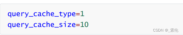
MySQL: What MySQL optimizations have you done?
2022强网杯 Quals Reverse 部分writeup
LeetCode每日两题01:移动零 (均1200道)方法:双指针
2022.8.9考试游记总结
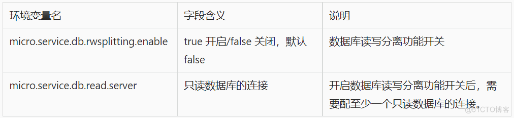
数据库治理利器:动态读写分离
2022.8.8 Exam area link (district) questions
Deep Learning (5) CNN Convolutional Neural Network
excel高级绘图技巧100讲(二十三)-Excel中实现倒计时计数
2022.8.8考试摄像师老马(photographer)题解
《GB39707-2020》PDF下载
【图像分类】2022-CycleMLP ICLR
[Kali Security Penetration Testing Practice Tutorial] Chapter 6 Password Attack
【红队】ATT&CK - 自启动 - 注册表运行键、启动文件夹
【Kali安全渗透测试实践教程】第8章 Web渗透
How Microbes Affect Physical Health
控制台中查看莫格命令的详细信息
Go语言JSON文件的读写操作