当前位置:网站首页>Machine learning practice - naive Bayes
Machine learning practice - naive Bayes
2022-04-23 18:34:00 【Xuanche_】

Naive Bayes
One 、 summary
Bayesian classification algorithm is a probabilistic classification method of statistics , Naive Bayesian classification is the simplest of Bayesian classification . The classification principle is to use Bayesian formula to calculate the posterior probability according to the prior probability of a feature , Then, the class with the maximum a posteriori probability is selected as the class to which the feature belongs . And
So it's called ” simple ”, Because Bayesian classification is only the most primitive 、 The simplest hypothesis : All features are statistically independent .
Suppose a sample X Yes a 1 {a}_{1} a1, a 2 {a}_{2} a2, a 3 {a}_{3} a3… a n {a}_{n} an Attributes , So there are P(X) = P( a 1 {a}_{1} a1, a 2 {a}_{2} a2… a n {a}_{n} an) =P( a 1 {a}_{1} a1)P( a 2 {a}_{2} a2)…*P( a n {a}_{n} an) Satisfying the sample formula means that the characteristic statistics are independent .
1. Conditional probability formula
Conditional probability (Condittional probability), It means in the event B When it happens , event A Probability of occurrence , use P(A|B) To express .

According to Wen's diagram : stay B In the event of an incident , event A The probability of occurrence is P(A∩B) Divide P(B)
P ( A ∣ B ) = P ( A ∩ B ) P ( B ) P(A|B)\, =\, \frac {P(A\cap B)} {P(B)} P(A∣B)=P(B)P(A∩B) ⇒ P ( A ∣ B ) P ( B ) = P ( A ∩ B ) P(A|B)\, P(B)=\, P(A\cap B) P(A∣B)P(B)=P(A∩B)
The same can be : P ( B ∣ A ) P ( A ) = P ( A ∩ B ) P(B|A)\, P(A)=\, P(A\cap B) P(B∣A)P(A)=P(A∩B)
therefore : P ( B ∣ A ) P ( A ) = P ( A ∣ B ) P ( B ) P(B|A)\, P(A)=\, P(A|B)P(B) P(B∣A)P(A)=P(A∣B)P(B) ⇒ P ( A ∣ B ) = P ( B ∣ A ) P ( A ) P ( B ) P(A|B)=\frac {P(B|A)P(A)} {P(B)} P(A∣B)=P(B)P(B∣A)P(A)
Then look at the full probability formula , If the event A 1 {A}_{1} A1, A 2 {A}_{2} A2,… A n {A}_{n} An Constitute a complete event with positive probability , So for any event B Then there are :
P ( B ) = P ( B A 1 ) + P ( B A 2 ) + . . . + P ( B A n ) P(B)\, =\, P(B{A}_{1})+P(B{A}_{2})+...+P(B{A}_{n}) P(B)=P(BA1)+P(BA2)+...+P(BAn)

P ( B ) = ∑ i = 1 n P ( A i ) P ( B ∣ A i ) P(B)\, =\, \sum ^{n}_{i=1} {P({
{A}_{i}}_{})P(B|{A}_{i})} P(B)=∑i=1nP(Ai)P(B∣Ai)
Bayesian judgment
According to the formula of conditional probability and total probability , The Bayesian formula can be obtained as follows :
P ( A ∣ B ) = P ( A ) P ( B ∣ A ) P ( B ) P(A|B)=P(A)\frac {P(B|A)} {P(B)} P(A∣B)=P(A)P(B)P(B∣A)
P ( A i ∣ B ) = P ( A i ) P ( B ∣ A ) ∑ i = 1 n P ( A i ) P ( B ∣ A i ) P({A}_{i}|B)=P({A}_{i})\frac {P(B|A)} {\sum ^{n}_{i=1} {P({A}_{i})P(B|{A}_{i})}} P(Ai∣B)=P(Ai)∑i=1nP(Ai)P(B∣Ai)P(B∣A)
P(A) be called " Prior probability "(Prior probability), That is to say B Before the incident , We are right. A The probability of an event .
P(A|B) be called " Posterior probability "(Posterior probability), That is to say B After the event , We are right. A Reassessment of event probabilities .
P(B|A)/P(B) be called " Possibility function "(Likely hood), This is an adjustment factor , Make the estimated probability closer to the real probability .
So conditional probability can be understood as : Posterior probability = Prior probability * Adjustment factor
If " Possibility function ">1, signify " Prior probability " Enhanced , event A More likely to happen ;
If " Possibility function "=1, signify B Events do not help to judge events A The possibility of ;
If " Possibility function "<1, signify " Prior probability " Weakened , event A Less likely .
Naive Bayes species
stay scikit-learn in , Altogether 3 A naive Bayesian classification algorithm .
Namely GaussianNB,MultinomialNB and BernoulliNB.
1. GaussianNB
GaussianNB A priori is ** Gaussian distribution ( Normal distribution ) Naive Bayes **, Assume that the data of each tag follows a simple normal distribution .
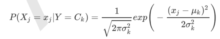
among by Y Of the k Class category . and For the values that need to be estimated from the training set .
here , use scikit-learn It's a simple implementation GaussianNB.
# Import package
import pandas as pd
from sklearn.naive_bayes import GaussianNB
from sklearn.model_selection import train_test_split
from sklearn.metrics import accuracy_score
# Import dataset
from sklearn import datasets
iris=datasets.load_iris()
# Sharding data sets
Xtrain, Xtest, ytrain, ytest = train_test_split(iris.data,
                                                iris.target,
                                                random_state=12)
# modeling
clf = GaussianNB()
clf.fit(Xtrain, ytrain)

# Perform prediction on the test set ,proba Derived is the probability that each sample belongs to a certain class
clf.predict(Xtest)
clf.predict_proba(Xtest)

# Test accuracy
accuracy_score(ytest, clf.predict(Xtest))
MultinomialNB
MultinomialNB Is a naive Bayes with a priori polynomial distribution . It assumes that the feature is generated by a simple polynomial distribution . Multinomial distribution can
Describe the probability of occurrence of various types of samples , Therefore, polynomial naive Bayes is very suitable for describing the characteristics of the number of occurrences or the proportion of occurrences .
This model is often used in text classification , The feature represents the number of times , For example, the number of occurrences of a word .
The polynomial distribution formula is as follows :
P ( X j = x j ∣ Y = C k ) = x j l + ξ m k + n ξ P({X}_{j}={x}_{j}|Y={C}_{k})=\frac { {x}_{jl\, }+ξ} { {m}_{k}+nξ} P(Xj=xj∣Y=Ck)=mk+nξxjl+ξ
among , P ( X j = x j ∣ Y = C k ) P({X}_{j}={x}_{j}|Y={C}_{k}) P(Xj=xj∣Y=Ck) It's No k Of categories j The number of dimensional features l The probability of the value conditions . m k {m}_{k} mk It's the output of training concentration k A sample of class
Count . ξ For a greater than 0 The constant , Often taken as 1, Laplace smoothing . You can also take other values .
BernoulliNB
BernoulliNB Is the naive Bayes with Bernoulli distribution a priori . Suppose that the prior probability of the feature is a binary Bernoulli distribution , It's like the following :

here There are only two values . x j l {x}_{jl} xjl Only value 0 perhaps 1.
In the Bernoulli model , The value of each feature is Boolean , namely true and false, perhaps 1 and 0.
In text classification , Is whether a feature appears in a document .
summary
- Generally speaking , If the distribution of sample characteristics is mostly continuous , Use GaussianNB It will be better. .
- If the distribution of sample features is mostly multivariate discrete values , Use MultinomialNB More appropriate .
- If the sample feature is binary discrete value or very sparse multivariate discrete value , You should use BernoulliNB.
版权声明
本文为[Xuanche_]所创,转载请带上原文链接,感谢
https://yzsam.com/2022/04/202204231824246309.html
边栏推荐
- QT tablewidget insert qcombobox drop-down box
- How to ensure the security of futures accounts online?
- 【ACM】376. Swing sequence
- STM32学习记录0008——GPIO那些事1
- 使用 bitnami/postgresql-repmgr 镜像快速设置 PostgreSQL HA
- QT error: no matching member function for call to ‘connect‘
- Custom prompt box MessageBox in QT
- Gson fastjason Jackson of object to JSON difference modifies the field name
- How to virtualize the video frame and background is realized in a few simple steps
- JD freefuck Jingdong HaoMao control panel background Command Execution Vulnerability
猜你喜欢

机器学习理论之(8):模型集成 Ensemble Learning
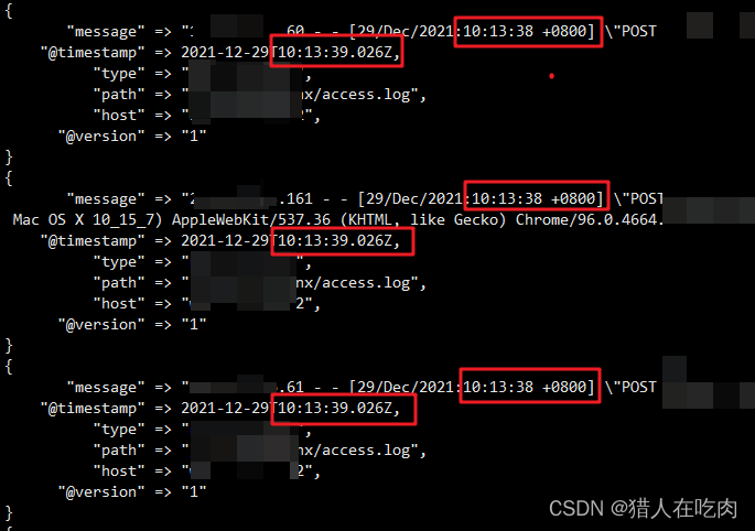
logstash 7. There is a time problem in X. the difference between @ timestamp and local time is 8 hours

【ACM】70. climb stairs
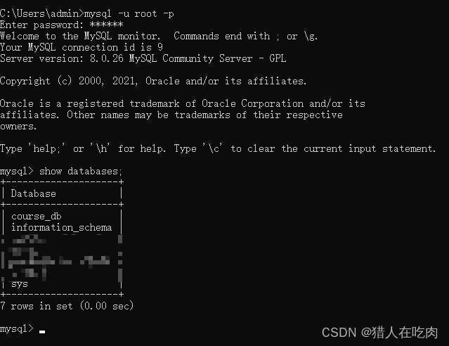
How to restore MySQL database after win10 system is reinstalled (mysql-8.0.26-winx64. Zip)

Query the logistics update quantity according to the express order number

From introduction to mastery of MATLAB (2)
QT add external font ttf
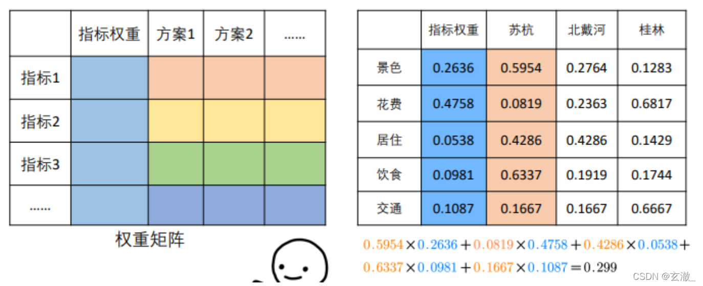
【数学建模】—— 层次分析法(AHP)
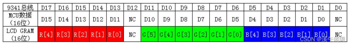
STM32: LCD display
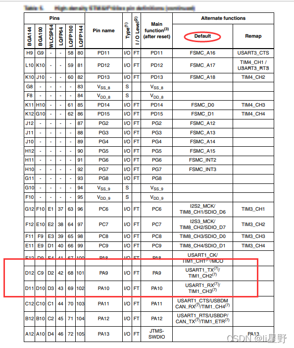
STM32学习记录0008——GPIO那些事1
随机推荐
Analysez l'objet promise avec le noyau dur (Connaissez - vous les sept API communes obligatoires et les sept questions clés?)
With the use of qchart, the final UI interface can be realized. The control of qweight can be added and promoted to a user-defined class. Only the class needs to be promoted to realize the coordinate
Database computer experiment 4 (data integrity and stored procedure)
The vivado project corresponding to the board is generated by TCL script
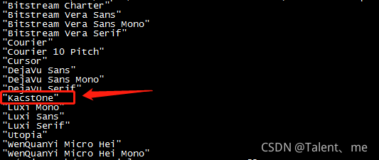
PowerDesigner various font settings; Preview font setting; SQL font settings
Use stm32cube MX / stm32cube ide to generate FatFs code and operate SPI flash
K210串口通信
Spark performance optimization guide
关于unity文件读取的操作(一)
Setting up keil environment of GD single chip microcomputer
Daily CISSP certification common mistakes (April 19, 2022)
QT reading and writing XML files (including source code + comments)
CISSP certified daily knowledge points (April 11, 2022)
QT excel operation summary
Halo 开源项目学习(七):缓存机制
机器学习理论之(8):模型集成 Ensemble Learning
【ACM】70. 爬楼梯
Resolves the interface method that allows annotation requests to be written in postman
串口调试工具cutecom和minicom
Software test summary