当前位置:网站首页>时序模型:门控循环单元网络(GRU)
时序模型:门控循环单元网络(GRU)
2022-04-23 15:36:00 【HadesZ~】
1. 模型定义
门控循环单元网络(Gated Recurrent Unit,GRU)1是在LSTM基础上发展而来的一种简化变体,它通常能以更快的计算速度达到与LSTM模型相似的效果2。
2. 模型结构与前向传播公式
GRU模型的隐藏状态计算模块不引入额外的记忆单元,且将逻辑门简化为重置门(reset gate)和更新门(update gate),其结构示意图及前向传播公式如下所示:
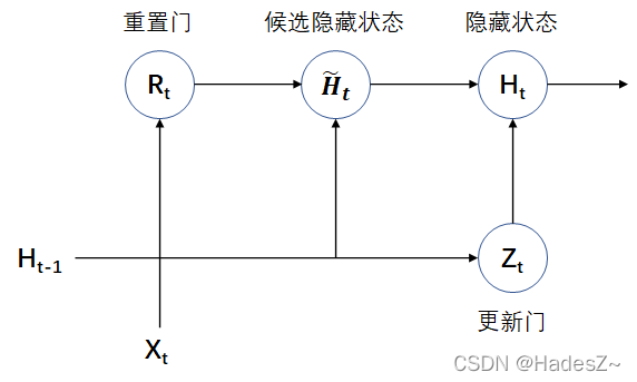
{ 输 入 : X t ∈ R m × d , H t − 1 ∈ R m × h 重 置 门 : R t = σ ( X t W x r + H t − 1 W h r + b r ) , W x r ∈ R d × h , W h r ∈ R h × h 候 选 隐 藏 状 态 : H ~ t = t a n h ( X t W x h + ( R t ⊙ H t − 1 ) W h h + b h ) , W x h ∈ R d × h , W h h ∈ R h × h 更 新 门 : Z t = σ ( X t W x z + H t − 1 W h z + b z ) , W x z ∈ R d × h , W h z ∈ R h × h 隐 藏 状 态 : H t = Z t ⊙ H t − 1 + ( 1 − Z t ) ⊙ H ~ t 输 出 : Y ^ t = H t W h y + b y , W h y ∈ R h × q 损 失 函 数 : L = ∑ t = 1 T l ( ( ^ Y ) t , Y t ) (2.1) \begin{cases} 输入: & X_t \in R^{m \times d}, \ \ \ \ H_{t-1} \in R^{m \times h} \\ \\ 重置门: & R_t = \sigma(X_tW_{xr} + H_{t-1}W_{hr} + b_r), & W_{xr} \in R^{d \times h},\ \ W_{hr} \in R^{h \times h} \\ \\ 候选隐藏状态: & \tilde{H}_t = tanh(X_tW_{xh} + (R_t \odot H_{t-1})W_{hh} + b_h),\ \ & W_{xh} \in R^{d \times h},\ \ W_{hh} \in R^{h \times h} \\ \\ 更新门: & Z_t = \sigma(X_tW_{xz} + H_{t-1}W_{hz} + b_z), & W_{xz} \in R^{d \times h},\ \ W_{hz} \in R^{h \times h} \\ \\ 隐藏状态: & H_t = Z_t \odot H_{t-1} + (1-Z_t) \odot \tilde{H}_t \\ \\ 输出: & \hat{Y}_t = H_tW_{hy} + b_y, & W_{hy} \in R^{h \times q} \\ \\ 损失函数: & L = \sum_{t=1}^{T} l(\hat(Y)_t, Y_t) \end{cases} \tag{2.1} ⎩⎪⎪⎪⎪⎪⎪⎪⎪⎪⎪⎪⎪⎪⎪⎪⎪⎪⎪⎪⎪⎪⎪⎪⎪⎪⎨⎪⎪⎪⎪⎪⎪⎪⎪⎪⎪⎪⎪⎪⎪⎪⎪⎪⎪⎪⎪⎪⎪⎪⎪⎪⎧输入:重置门:候选隐藏状态:更新门:隐藏状态:输出:损失函数:Xt∈Rm×d, Ht−1∈Rm×hRt=σ(XtWxr+Ht−1Whr+br),H~t=tanh(XtWxh+(Rt⊙Ht−1)Whh+bh), Zt=σ(XtWxz+Ht−1Whz+bz),Ht=Zt⊙Ht−1+(1−Zt)⊙H~tY^t=HtWhy+by,L=∑t=1Tl((^Y)t,Yt)Wxr∈Rd×h, Whr∈Rh×hWxh∈Rd×h, Whh∈Rh×hWxz∈Rd×h, Whz∈Rh×hWhy∈Rh×q(2.1)
3. GRU的反向传播过程
因未引入额外的记忆单元,所以GRU反向传播的计算图与RNN一致(如作者文章:时序模型:循环神经网络(RNN)中图3所示),GRU的反向传播公式如下所示:
∂ L ∂ Y ^ t = ∂ l ( Y ^ t , Y t ) T ⋅ ∂ Y ^ t (3.1) \frac{\partial L}{\partial \hat{Y}_t} = \frac{\partial l(\hat{Y}_t, Y_t)}{T \cdot\partial \hat{Y}_t} \tag {3.1} ∂Y^t∂L=T⋅∂Y^t∂l(Y^t,Yt)(3.1)
∂ L ∂ Y ^ t ⇒ { ∂ L ∂ W h y = ∂ L ∂ Y ^ t ∂ Y ^ t ∂ W h y ∂ L ∂ H t = { ∂ L ∂ Y ^ t ∂ Y ^ t ∂ H t , t = T ∂ L ∂ Y ^ t ∂ Y ^ t ∂ H t + ∂ L ∂ H t + 1 ∂ H t + 1 ∂ H t , t < T (3.2) \frac{\partial L}{\partial \hat{Y}_t} \Rightarrow \begin{cases} \frac{\partial L}{\partial W_{hy}} = \frac{\partial L}{\partial \hat{Y}_t} \frac{\partial \hat{Y}_t}{\partial W_{hy}} \\ \\ \frac{\partial L}{\partial H_t} = \begin{cases} \frac{\partial L}{\partial \hat{Y}_t} \frac{\partial \hat{Y}_t}{\partial H_t}, & t=T \\ \\ \frac{\partial L}{\partial \hat{Y}_t} \frac{\partial \hat{Y}_t}{\partial H_t} + \frac{\partial L}{\partial H_{t+1}}\frac{\partial H_{t+1}}{\partial H_{t}}, & t<T \end{cases} \end{cases} \tag {3.2} ∂Y^t∂L⇒⎩⎪⎪⎪⎪⎪⎪⎪⎨⎪⎪⎪⎪⎪⎪⎪⎧∂Why∂L=∂Y^t∂L∂Why∂Y^t∂Ht∂L=⎩⎪⎪⎨⎪⎪⎧∂Y^t∂L∂Ht∂Y^t,∂Y^t∂L∂Ht∂Y^t+∂Ht+1∂L∂Ht∂Ht+1,t=Tt<T(3.2)
{ ∂ L ∂ W x z = ∂ L ∂ Z t ∂ Z t ∂ W x z ∂ L ∂ W h z = ∂ L ∂ Z t ∂ Z t ∂ W h z ∂ L ∂ b z = ∂ L ∂ Z t ∂ Z t ∂ b z { ∂ L ∂ W x h = ∂ L ∂ H ~ t ∂ H ~ t ∂ W x h ∂ L ∂ W h h = ∂ L ∂ H ~ t ∂ H ~ t ∂ W h h ∂ L ∂ b h = ∂ L ∂ H ~ t ∂ H ~ t ∂ b h (3.3) \begin{matrix} \begin{cases} \frac{\partial L}{\partial W_{xz}} = \frac{\partial L}{\partial Z_{t}}\frac{\partial Z_{t}}{\partial W_{xz}} \\ \\ \frac{\partial L}{\partial W_{hz}} = \frac{\partial L}{\partial Z_{t}}\frac{\partial Z_{t}}{\partial W_{hz}} \\ \\ \frac{\partial L}{\partial b_{z}} = \frac{\partial L}{\partial Z_{t}}\frac{\partial Z_{t}}{\partial b_{z}} \end{cases} & & & & \begin{cases} \frac{\partial L}{\partial W_{xh}} = \frac{\partial L}{\partial \tilde{H}_t}\frac{\partial \tilde{H}_t}{\partial W_{xh}} \\ \\ \frac{\partial L}{\partial W_{hh}} = \frac{\partial L}{\partial \tilde{H}_t}\frac{\partial \tilde{H}_t}{\partial W_{hh}} \\ \\ \frac{\partial L}{\partial b_{h}} = \frac{\partial L}{\partial \tilde{H}_t}\frac{\partial \tilde{H}_t}{\partial b_{h}} \end{cases} \end{matrix} \tag {3.3} ⎩⎪⎪⎪⎪⎪⎪⎨⎪⎪⎪⎪⎪⎪⎧∂Wxz∂L=∂Zt∂L∂Wxz∂Zt∂Whz∂L=∂Zt∂L∂Whz∂Zt∂bz∂L=∂Zt∂L∂bz∂Zt⎩⎪⎪⎪⎪⎪⎪⎪⎨⎪⎪⎪⎪⎪⎪⎪⎧∂Wxh∂L=∂H~t∂L∂Wxh∂H~t∂Whh∂L=∂H~t∂L∂Whh∂H~t∂bh∂L=∂H~t∂L∂bh∂H~t(3.3)
{ ∂ L ∂ W x r = ∂ L ∂ R t ∂ R t ∂ W x r ∂ L ∂ W h r = ∂ L ∂ R t ∂ R t ∂ W h r ∂ L ∂ b r = ∂ L ∂ R t ∂ R t ∂ b r (3.4) \begin{cases} \frac{\partial L}{\partial W_{xr}} = \frac{\partial L}{\partial R_{t}}\frac{\partial R_{t}}{\partial W_{xr}} \\ \\ \frac{\partial L}{\partial W_{hr}} = \frac{\partial L}{\partial R_{t}}\frac{\partial R_{t}}{\partial W_{hr}} \\ \\ \frac{\partial L}{\partial b_{r}} = \frac{\partial L}{\partial R_{t}}\frac{\partial R_{t}}{\partial b_{r}} \end{cases} \tag {3.4} ⎩⎪⎪⎪⎪⎪⎪⎨⎪⎪⎪⎪⎪⎪⎧∂Wxr∂L=∂Rt∂L∂Wxr∂Rt∂Whr∂L=∂Rt∂L∂Whr∂Rt∂br∂L=∂Rt∂L∂br∂Rt(3.4)
与LSTM同理,GRU反向传播公式求解的关键也是对不同时间步间(传递)梯度 的求解,其方法与LSTM一致本文不再赘述。且同样我们也可以得出定性结论,GRU缓解长期依赖问题的原理与LSTM类似,都是通过高阶幂次项乘数调控和添加低阶幂次项实现。其中,重置门有助于捕获序列中的短期依赖关系,更新门有助于捕获序列中的长期依赖关系。(具体请详见作者文章:时序模型:长短期记忆网络(LSTM)中的证明过程)
4. 模型的代码实现
4.1 TensorFlow 框架实现
4.2 Pytorch 框架实现
import torch
from torch import nn
from torch.nn import functional as F


#
class Dense(nn.Module):
    """ Args: outputs_dim: Positive integer, dimensionality of the output space. activation: Activation function to use. If you don't specify anything, no activation is applied (ie. "linear" activation: `a(x) = x`). use_bias: Boolean, whether the layer uses a bias vector. kernel_initializer: Initializer for the `kernel` weights matrix. bias_initializer: Initializer for the bias vector. Input shape: N-D tensor with shape: `(batch_size, ..., input_dim)`. The most common situation would be a 2D input with shape `(batch_size, input_dim)`. Output shape: N-D tensor with shape: `(batch_size, ..., units)`. For instance, for a 2D input with shape `(batch_size, input_dim)`, the output would have shape `(batch_size, units)`. """
    def __init__(self, input_dim, output_dim, **kwargs):
        super().__init__()
        # 超参定义
        self.use_bias = kwargs.get('use_bias', True)
        self.kernel_initializer = kwargs.get('kernel_initializer', nn.init.xavier_uniform_)
        self.bias_initializer = kwargs.get('bias_initializer', nn.init.zeros_)
        #
        self.Linear = nn.Linear(input_dim, output_dim, bias=self.use_bias)
        self.Activation = kwargs.get('activation', nn.ReLU())
        # 参数初始化
        self.kernel_initializer(self.Linear.weight)
        self.bias_initializer(self.Linear.bias)

    def forward(self, inputs):
        outputs = self.Activation(
            self.Linear(inputs)
        )
        return outputs


#
class GRU_Cell(nn.Module):
    def __init__(self, token_dim, hidden_dim
                 , reset_act=nn.ReLU()
                 , update_act=nn.ReLU()
                 , hathid_act=nn.Tanh()
                 , **kwargs):
        super().__init__()
        #
        self.hidden_dim = hidden_dim
        #
        self.ResetG = Dense(
            token_dim + self.hidden_dim, self.hidden_dim
            , activation=reset_act, **kwargs
        )
        self.UpdateG = Dense(
            token_dim + self.hidden_dim, self.hidden_dim
            , activation=update_act, **kwargs
        )
        self.HatHidden = Dense(
            token_dim + self.hidden_dim, self.hidden_dim
            , activation=hathid_act, **kwargs
        )

    def forward(self, inputs, last_state):
        last_hidden = last_state[-1]
        #
        Rg = self.ResetG(
            torch.concat([inputs, last_hidden], dim=1)
        )
        Zg = self.UpdateG(
            torch.concat([inputs, last_hidden], dim=1)
        )
        hat_hidden = self.HatHidden(
            torch.concat([inputs, Rg * last_hidden], dim=1)
        )
        hidden = Zg*last_hidden + (1-Zg)*hat_hidden
        #
        return [hidden]

    def zero_initialization(self, batch_size):
        return torch.zeros([batch_size, self.hidden_dim])


#
class RNN_Layer(nn.Module):
    def __init__(self, rnn_cell, bidirectional=False):
        super().__init__()
        self.RNNCell = rnn_cell
        self.bidirectional = bidirectional

    def forward(self, inputs, mask=None, initial_state=None):
        """ inputs: it's shape is [batch_size, time_steps, token_dim] mask: it's shape is [batch_size, time_steps] :return hidden_state_seqence: its' shape is [batch_size, time_steps, hidden_dim] last_state: it is the hidden state of input sequences at last time step, but, attentively, the last token wouble be a padding token, so this last state is not the real last state of input sequences; if you want to get the real last state of input sequences, please use utils.get_rnn_last_state(hidden_state_seqence). """
        batch_size, time_steps, token_dim = inputs.shape
        #
        if initial_state is None:
            initial_state = self.RNNCell.zero_initialization(batch_size)
        if mask is None:
            if batch_size == 1:
                mask = torch.ones([1, time_steps])
            else:
                raise ValueError('请给定掩码矩阵(mask)')

        # 正向时间步循环
        hidden_list = []
        hidden_state = initial_state
        for i in range(time_steps):
            hidden_state = self.RNNCell(inputs[:, i], hidden_state)
            hidden_list.append(hidden_state[-1])
            hidden_state = [hidden_state[j] * mask[:, i:i+1] + initial_state[j] * (1-mask[:, i:i+1])
                            for j in range(len(hidden_state))]  # 重新初始化(加数项作用)
        #
        seqences = torch.reshape(
            torch.unsqueeze(
                torch.concat(hidden_list, dim=1), dim=1
            )
            , [batch_size, time_steps, -1]
        )
        last_state = hidden_list[-1]

        # 反向时间步循环
        if self.bidirectional is True:
            hidden_list = []
            hidden_state = initial_state
            for i in range(time_steps, 0, -1):
                hidden_state = self.RNNCell(inputs[:, i-1], hidden_state)
                hidden_list.append(hidden_state[-1])
                hidden_state = [hidden_state[j] * mask[:, i-1:i] + initial_state[j] * (1 - mask[:, i-1:i])
                                for j in range(len(hidden_state))]  # 重新初始化(加数项作用)
            #
            seqences = torch.concat([
                seqences,
                torch.reshape(
                    torch.unsqueeze(
                        torch.concat(hidden_list, dim=1), dim=1)
                    , [batch_size, time_steps, -1])
                ]
                , dim=-1
            )
            last_state = torch.concat([
                last_state
                , hidden_list[-1]
                ]
                , dim=-1
            )

        return {

            'hidden_state_seqences': seqences
            , 'last_state': last_state
        }
Cho, K., Van Merriënboer, B., Bahdanau, D., & Bengio, Y. (2014). On the properties of neural machine translation: encoder-decoder approaches. arXiv preprint arXiv:1409.1259. ︎
Chung, J., Gulcehre, C., Cho, K., & Bengio, Y. (2014). Empirical evaluation of gated recurrent neural networks on sequence modeling. arXiv preprint arXiv:1412.3555. ︎
版权声明
本文为[HadesZ~]所创,转载请带上原文链接,感谢
https://blog.csdn.net/xunyishuai5020/article/details/123069473
边栏推荐
猜你喜欢
T2 icloud calendar cannot be synchronized
Squid agent
My raspberry PI zero 2W toss notes to record some problems and solutions
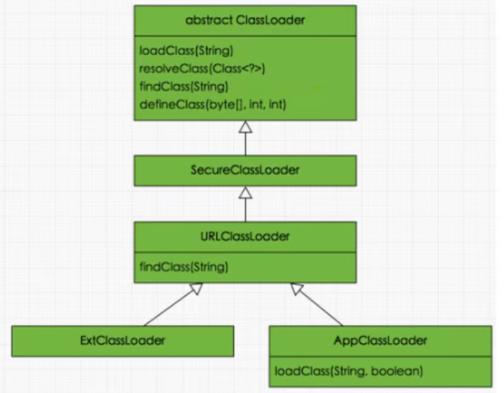
JVM-第2章-类加载子系统(Class Loader Subsystem)
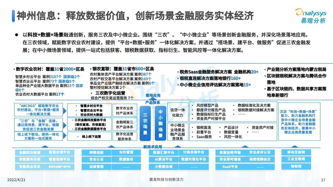
2022年中国数字科技专题分析

The wechat applet optimizes the native request through the promise of ES6
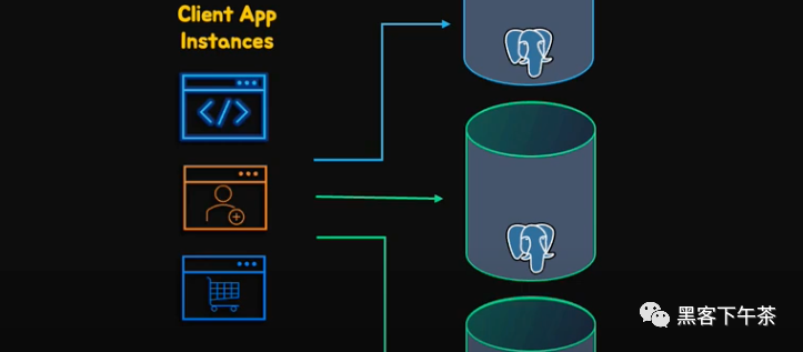
pgpool-II 4.3 中文手册 - 入门教程
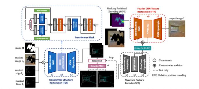
CVPR 2022 优质论文分享

考试考试自用

服务器中毒了怎么办?服务器怎么防止病毒入侵?
随机推荐
字节面试 transformer相关问题 整理复盘
regular expression
T2 icloud calendar cannot be synchronized
Connect PHP to MySQL via PDO ODBC
移动app软件测试工具有哪些?第三方软件测评小编分享
For examination
Mobile finance (for personal use)
Mysql连接查询详解
My raspberry PI zero 2W toss notes to record some problems and solutions
Cookie&Session
kubernetes之常用Pod控制器的使用
Baidu written test 2022.4.12 + programming topic: simple integer problem
Sword finger offer (2) -- for Huawei
Use of common pod controller of kubernetes
WPS品牌再升级专注国内,另两款国产软件低调出国门,却遭禁令
Summary of interfaces for JDBC and servlet to write CRUD
[backtrader source code analysis 18] Yahoo Py code comments and analysis (boring, interested in the code, you can refer to)
php类与对象
使用 Bitnami PostgreSQL Docker 镜像快速设置流复制集群
Adobe Illustrator menu in Chinese and English