当前位置:网站首页>R语言中实现作图对象排列的函数总结
R语言中实现作图对象排列的函数总结
2022-04-23 15:47:00 【zoujiahui_2018】
文章目录
par(mfrow=c(n,m))基础作图
par(mfrowc(n,m))是R基础作图中的函数,只对基础作图函数plot的对象起作用
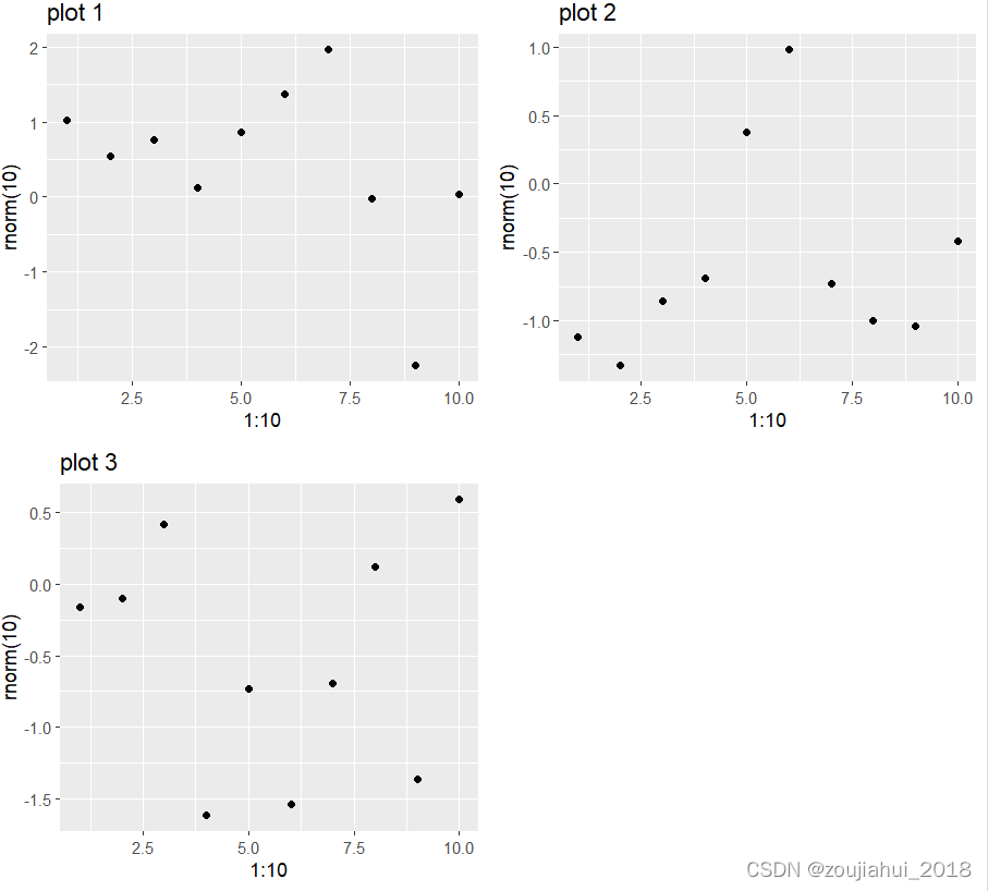
gridExtra::grid.arrange()针对ggplot对象
grid.arrange()函数只能用于对ggplot对象进行排布
用法
# 全部参数
grid.arrange(..., grobs = list(...), layout_matrix, vp = NULL,
  name = "arrange", as.table = TRUE, respect = FALSE, clip = "off",
  nrow = NULL, ncol = NULL, widths = NULL, heights = NULL, top = NULL,
  bottom = NULL, left = NULL, right = NULL, padding = unit(0.5, "line"),newpage=TRUE)

#常用格式
grid.arrange(p1,p2,p3,...,ncol=n,nrow=m)
实例
library(gridExtra)
library(ggplot2)
p1=qplot(1:10, rnorm(10), main=paste("plot", 1))
p2=qplot(1:10, rnorm(10), main=paste("plot", 2))
p3=qplot(1:10, rnorm(10), main=paste("plot", 3))
grid.arrange(p1,p2,p3,nrow=2,ncol=2)
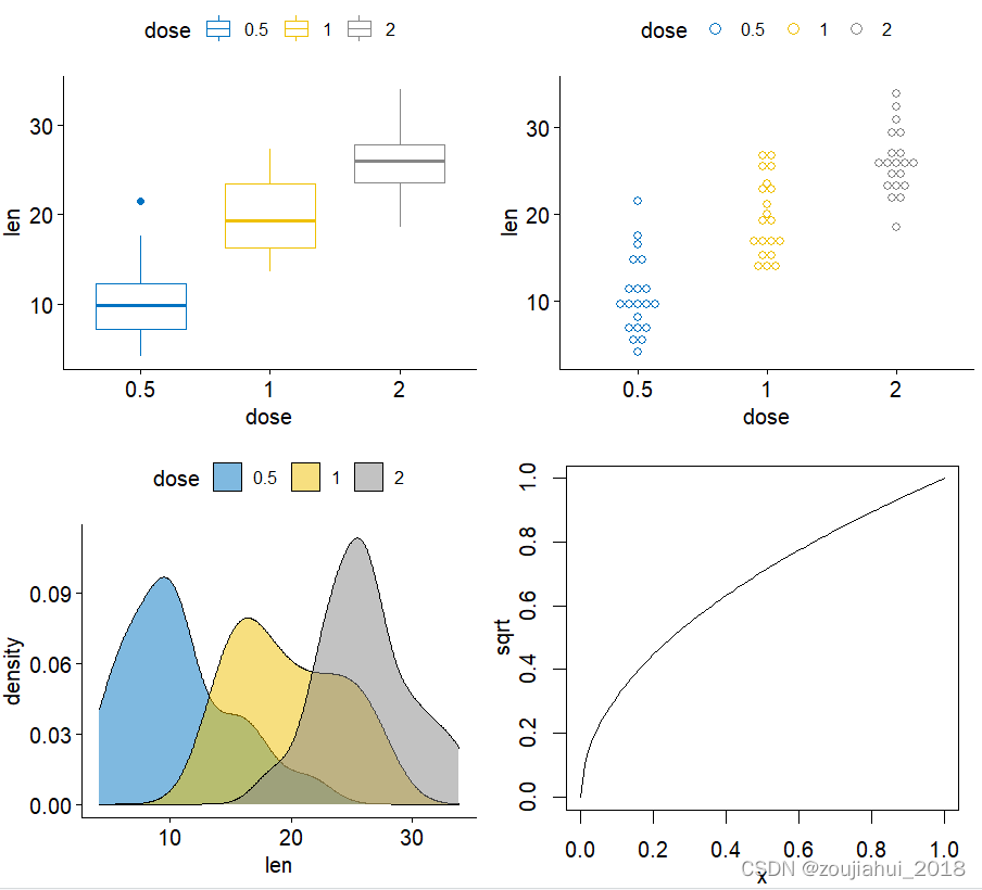
ggpubr::ggarrange()可处理ggplot对象和基础plot对象
用法
ggarrange(
  ...,
  plotlist = NULL,
  ncol = NULL,
  nrow = NULL,
  labels = NULL,
  label.x = 0,
  label.y = 1,
  hjust = -0.5,
  vjust = 1.5,
  font.label = list(size = 14, color = "black", face = "bold", family = NULL),
  align = c("none", "h", "v", "hv"),
  widths = 1,
  heights = 1,
  legend = NULL,
  common.legend = FALSE,
  legend.grob = NULL
)
实例
library(ggplot2)
library(ggpubr)
data("ToothGrowth")
df <- ToothGrowth
df$dose <- as.factor(df$dose)

bxp <- ggboxplot(df, x = "dose", y = "len",
                 color = "dose", palette = "jco")
dp <- ggdotplot(df, x = "dose", y = "len",
                color = "dose", palette = "jco")
dens <- ggdensity(df, x = "len", fill = "dose", palette = "jco")


plt<- ~{

    par(
      mar = c(3, 3, 1, 1),
      mgp = c(2, 1, 0)
    )
    plot(sqrt)
  }

# Arrange
# ::::::::::::::::::::::::::::::::::::::::::::::::::
ggarrange(bxp, dp,dens,plt, ncol = 2, nrow = 2)
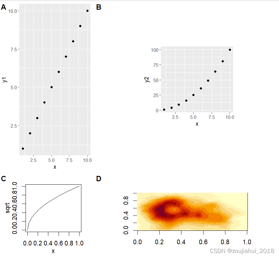
cowplot::plot_grid()可以用于不同对象
用法
plot_grid(
  ...,
  plotlist = NULL,
  align = c("none", "h", "v", "hv"),
  axis = c("none", "l", "r", "t", "b", "lr", "tb", "tblr"),
  nrow = NULL,
  ncol = NULL,
  rel_widths = 1,
  rel_heights = 1,
  labels = NULL,
  label_size = 14,
  label_fontfamily = NULL,
  label_fontface = "bold",
  label_colour = NULL,
  label_x = 0,
  label_y = 1,
  hjust = -0.5,
  vjust = 1.5,
  scale = 1,
  greedy = TRUE,
  byrow = TRUE,
  cols = NULL,
  rows = NULL
)
实例
library(ggplot2)
library(cowplot)
df <- data.frame(
x = 1:10, y1 = 1:10, y2 = (1:10)^2, y3 = (1:10)^3, y4 = (1:10)^4
)
p1 <- ggplot(df, aes(x, y1)) + geom_point()
p2 <- ggplot(df, aes(x, y2)) + geom_point()
p6 <- ~{
par(
mar = c(3, 3, 1, 1),
mgp = c(2, 1, 0)
)
plot(sqrt)
}
p7 <- function() {
par(
mar = c(2, 2, 1, 1),
mgp = c(2, 1, 0)
)
image(volcano)
}
# ggarrange(p1,p2,p3,p4)
# making rows and columns of different widths/heights
plot_grid(
p1, p2,p6,p7, nrow = 2,ncol=2,rel_heights = c(2,1), rel_widths = c(1, 2),labels = "AUTO",scale = c(1, .5, .9, .7)
)
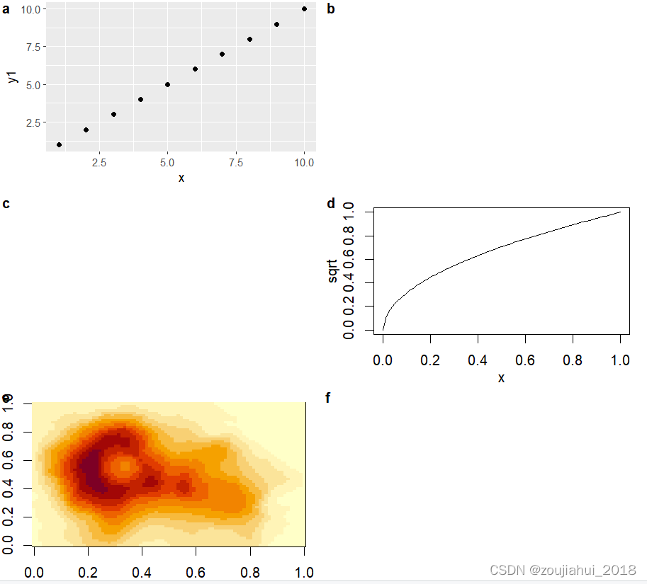
#' # missing plots in some grid locations, auto-generate lower-case labels
plot_grid(
p1, NULL, NULL, p6, p7, NULL,
ncol = 2,
labels = "auto",
label_size = 12,
align = "v"
)
customLayout::lay_new()功能更加强大灵活
未完待续…
版权声明
本文为[zoujiahui_2018]所创,转载请带上原文链接,感谢
https://blog.csdn.net/qq_18055167/article/details/124337417
边栏推荐
猜你喜欢
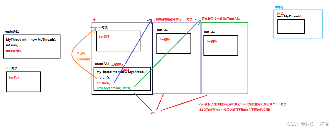
多线程原理和常用方法以及Thread和Runnable的区别
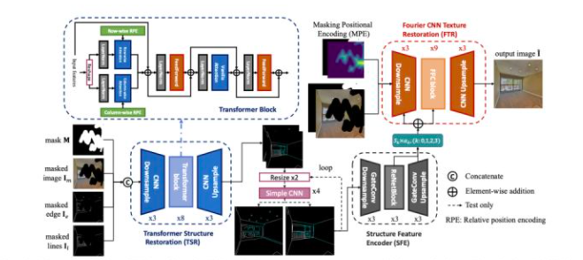
CVPR 2022 优质论文分享
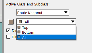
cadence SPB17. 4 - Active Class and Subclass
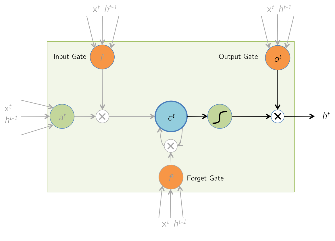
Temporal model: long-term and short-term memory network (LSTM)

Load Balancer

网站建设与管理的基本概念
Modèle de Cluster MySQL et scénario d'application

Metalife established a strategic partnership with ESTV and appointed its CEO Eric Yoon as a consultant
Single architecture system re architecture
![[AI weekly] NVIDIA designs chips with AI; The imperfect transformer needs to overcome the theoretical defect of self attention](/img/bf/2b4914276ec1083df697383fec8f22.png)
[AI weekly] NVIDIA designs chips with AI; The imperfect transformer needs to overcome the theoretical defect of self attention
随机推荐
服务器中毒了怎么办?服务器怎么防止病毒入侵?
时序模型:长短期记忆网络(LSTM)
贫困的无网地区怎么有钱建设网络?
leetcode-374 猜数字大小
单体架构系统重新架构
Application of Bloom filter in 100 million flow e-commerce system
One brush 314 sword finger offer 09 Implement queue (E) with two stacks
移动金融(自用)
PHP classes and objects
JVM-第2章-类加载子系统(Class Loader Subsystem)
[backtrader source code analysis 18] Yahoo Py code comments and analysis (boring, interested in the code, you can refer to)
How can poor areas without networks have money to build networks?
pywintypes.com_error: (-2147221020, ‘无效的语法‘, None, None)
多级缓存使用
The length of the last word of the string
Code live collection ▏ software test report template Fan Wen is here
基础贪心总结
大厂技术实现 | 行业解决方案系列教程
Spark 算子之sortBy使用
Go并发和通道