深度学习100例 | 第41天-卷积神经网络（CNN）：UrbanSound8K音频分类（语音识别）

• 运行环境：python3
• 作者：K同学啊
• 选自专栏：《深度学习100例》
• 精选专栏：《新手入门深度学习》
• 推荐专栏：《Matplotlib教程》
• 🧿 优秀专栏：《Python入门100题》

---

我的环境：

• 语言环境：Python3.6.5
• 编译器：jupyter notebook
• 深度学习环境：TensorFlow2.4.1
• 显卡（GPU）：NVIDIA GeForce RTX 3080
• 数据地址：【传送门】

我们的代码流程图如下所示：

一、准备工作

大家好，我是K同学啊！

今天给大家分享一个音频分类的实战案例。

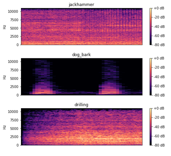
使用的数据集为UrbanSound8K，该数据集包含来自 10 个类别的城市声音的 8732 个标记声音摘录 (<=4s)：air_conditioner、car_horn、children_playing、dog_bark、drilling、enginge_idling、gun_shot、jackhammer、siren和 street_music，数据分别存在fold1-fold10等十个文件夹中。

除了声音摘录之外，还提供了一个 CSV 文件，其中包含有关每个摘录的元数据。

方法介绍

1. 有 3 种从音频文件中提取特征的基本方法：

   a) 使用音频文件的 mffcs 数据
   b) 使用音频的频谱图图像，然后将其转换为数据点（就像对图像所做的那样）。这可以使用 Librosa 的 mel_spectogram 函数 轻松完成
   c) 结合这两个特征来构建更好的模型。 （需要大量时间来读取和提取数据）。

2. 我选择使用第二种方法。

3. 标签已转换为分类数据以进行分类。

4. CNN 已被用作对数据进行分类的主要层

1. 导入所需的库

# Basic Libraries

import pandas as pd
import numpy as np

pd.plotting.register_matplotlib_converters()
import matplotlib.pyplot as plt
%matplotlib inline
import seaborn as sns

from sklearn.model_selection import train_test_split
from sklearn.metrics import classification_report
from sklearn.model_selection import GridSearchCV
from sklearn.preprocessing import MinMaxScaler
from tensorflow.keras.models import Sequential
from tensorflow.keras.layers import Conv2D, Flatten, Dense, MaxPool2D, Dropout
from tensorflow.keras.utils import to_categorical 
import os,glob,skimage,librosa
import librosa.display

import warnings
warnings.filterwarnings("ignore")             #忽略警告信息

2. 分析数据类型及格式

分析CSV数据

df = pd.read_csv("./41-data/UrbanSound8K.csv")

df.head()

	slice_file_name	fsID	start	end	salience	fold	classID	class
0	100032-3-0-0.wav	100032	0.0	0.317551	1	5	3	dog_bark
1	100263-2-0-117.wav	100263	58.5	62.500000	1	5	2	children_playing
2	100263-2-0-121.wav	100263	60.5	64.500000	1	5	2	children_playing
3	100263-2-0-126.wav	100263	63.0	67.000000	1	5	2	children_playing
4	100263-2-0-137.wav	100263	68.5	72.500000	1	5	2	children_playing

列名

• slice_file_name：音频文件名字. 命名格式为: [fsID]-[classID]-[occurrenceID]-[sliceID].wav

  • [fsID]：从中提取摘录（片段）的录音的 Freesound ID
  • [classID]：类别ID
  • [occurrenceID]：一个数字标识符，用于区分原始录音中不同事件的声音
  • [sliceID]：一个数字标识符，用于区分从同一事件中获取的不同切片

• fsID：从中提取摘录（片段）的录音的 Freesound ID

• start：原始 Freesound 录音中片段的开始时间

• end：原始Freesound录音中切片的结束时间

• salience：声音的（主观）显着性等级。 1 = 前景，2 = 背景。

• fold：一共1-10,10个文件夹

• classID：声音类别的数字标识符：

  • 0 = air_conditioner
  • 1 = car_horn
  • 2 = children_playing
  • 3 = dog_bark
  • 4 = drilling
  • 5 = engine_idling
  • 6 = gun_shot
  • 7 = jackhammer
  • 8 = siren
  • 9 = street_music

使用Librosa分析随机声音样本

a,b = librosa.load()返回值：

• a: 音频的信号值，类型是ndarray
• b: 采样率

3. 数据展示

import IPython.display as ipd
ipd.Audio('./41-data/fold5/100263-2-0-117.wav')

dataSample, sampling_rate = librosa.load('./41-data/fold5/100032-3-0-0.wav')

plt.figure(figsize=(10, 3))

D = librosa.amplitude_to_db(np.abs(librosa.stft(dataSample)), ref=np.max)
librosa.display.specshow(D, y_axis='linear')

plt.colorbar(format='%+2.0f dB')
plt.title('Linear-frequency power spectrogram')
plt.show()

arr  = np.array(df["slice_file_name"])
fold = np.array(df["fold"])
cla  = np.array(df["class"])

for i in range(192, 197, 2):
    plt.figure(figsize=(8, 2))
    
    path = './41-data/fold' + str(fold[i]) + '/' + arr[i]
    data, sampling_rate = librosa.load(path)
    
    D = librosa.amplitude_to_db(np.abs(librosa.stft(data)), ref=np.max)
    librosa.display.specshow(D, y_axis='linear')
    plt.colorbar(format='%+2.0f dB')
    plt.title(cla[i])

二、特征提取与数据集构建

先看一下使用librosa.feature.melspectrogram()函数提取出来的数据shape

arr = librosa.feature.melspectrogram(y=data, sr=sampling_rate)
arr.shape

(128, 173)

1. 数据特征提取

feature = []
label   = []

def parser():
    # 加载文件并提取特征
    for i in range(8732):
        if i%1000 == 0:
            print("已经提取%d份数据特征"%i)
            
        file_name = './41-data/fold' + str(df["fold"][i]) + '/' + df["slice_file_name"][i]
        X, sample_rate = librosa.load(file_name, res_type='kaiser_fast') 
        # 提取频谱图形成图像数组
        mels = np.mean(librosa.feature.melspectrogram(y=X, sr=sample_rate).T,axis=0)        
        feature.append(mels)
        label.append(df["classID"][i])
    print("数据特征提取完成！")
    return [feature, label]

temp = parser()

已经提取0份数据特征
已经提取1000份数据特征
已经提取2000份数据特征
已经提取3000份数据特征
已经提取4000份数据特征
已经提取5000份数据特征
已经提取6000份数据特征
已经提取7000份数据特征
已经提取8000份数据特征
数据特征提取完成！

temp_numpy = np.array(temp).transpose()

X_ = temp_numpy[:, 0]
Y_ = temp_numpy[:, 1]

X = np.array([X_[i] for i in range(8732)])
Y = to_categorical(Y_)

print(X.shape, Y.shape)

(8732, 128) (8732, 10)

2. 数据集构建

X_train, X_test, Y_train, Y_test = train_test_split(X, Y, random_state = 1)

X_train = X_train.reshape(6549, 16, 8, 1)
X_test  = X_test.reshape(2183, 16, 8, 1)

input_dim = (16, 8, 1)

三、构建模型并训练

model = Sequential()

model.add(Conv2D(64, (3, 3), padding = "same", activation = "tanh", input_shape = input_dim))
model.add(MaxPool2D(pool_size=(2, 2)))
model.add(Conv2D(128, (3, 3), padding = "same", activation = "tanh"))
model.add(MaxPool2D(pool_size=(2, 2)))
model.add(Dropout(0.1))
model.add(Flatten())
model.add(Dense(1024, activation = "tanh"))
model.add(Dense(10, activation = "softmax"))

model.compile(optimizer = 'adam', loss = 'categorical_crossentropy', metrics = ['accuracy'])

model.fit(X_train, Y_train, epochs = 90, batch_size = 50, validation_data = (X_test, Y_test))

Epoch 1/90
131/131 [==============================] - 3s 4ms/step - loss: 1.5368 - accuracy: 0.4717 - val_loss: 1.3617 - val_accuracy: 0.5144
Epoch 2/90
131/131 [==============================] - 0s 2ms/step - loss: 1.1502 - accuracy: 0.6091 - val_loss: 1.1119 - val_accuracy: 0.6326
  ......
131/131 [==============================] - 0s 2ms/step - loss: 0.0481 - accuracy: 0.9835 - val_loss: 0.8535 - val_accuracy: 0.8653
Epoch 89/90
131/131 [==============================] - 0s 2ms/step - loss: 0.0511 - accuracy: 0.9818 - val_loss: 0.7716 - val_accuracy: 0.8694
Epoch 90/90
131/131 [==============================] - 0s 2ms/step - loss: 0.0502 - accuracy: 0.9829 - val_loss: 0.8673 - val_accuracy: 0.8630

model.summary()

Model: "sequential"
_________________________________________________________________
Layer (type)                 Output Shape              Param #   
=================================================================
conv2d (Conv2D)              (None, 16, 8, 64)         640       
_________________________________________________________________
max_pooling2d (MaxPooling2D) (None, 8, 4, 64)          0         
_________________________________________________________________
conv2d_1 (Conv2D)            (None, 8, 4, 128)         73856     
_________________________________________________________________
max_pooling2d_1 (MaxPooling2 (None, 4, 2, 128)         0         
_________________________________________________________________
dropout (Dropout)            (None, 4, 2, 128)         0         
_________________________________________________________________
flatten (Flatten)            (None, 1024)              0         
_________________________________________________________________
dense (Dense)                (None, 1024)              1049600   
_________________________________________________________________
dense_1 (Dense)              (None, 10)                10250     
=================================================================
Total params: 1,134,346
Trainable params: 1,134,346
Non-trainable params: 0
_________________________________________________________________

predictions = model.predict(X_test)
score = model.evaluate(X_test, Y_test)
print(score)

69/69 [==============================] - 0s 1ms/step - loss: 0.8673 - accuracy: 0.8630
[0.8672816753387451, 0.8630325198173523]