本文整理自《Python机器学习》

决策树

The decision tree can be seen as data from a top-down partitioning method,Usually in the form of binary tree.
通过决策树算法,从树根开始,Based on the available maximum信息增益（Information Gain, IG）The characteristics of the data is divided into.
Objective function can be implemented in each division of the maximization of information gain,其定义如下：
$$\text{IG}(D_p,f)=I(D_p)-\sum _{j=1}^m\frac{N_j}{N_p}I(D_j)$$
其中$f$To be divided by the characteristics of the,$D_p$与$D_j$Parent node respectively and the first$j$个子节点,$I$For purity criteria,$N_p$For the parent sample size,$N_j$为第$j$The number of child nodes in the sample.The type indicates that,Information gain is not purity of the parent node with the difference between the sum of all child nodes don't purity,Child node of the impurity of the lower,信息增益越大.
对于二叉树（scikit-learn中的实现方式）有：
$$\text{IG}(D_p,a)=I(D_p)-\frac{N_{left}}{N_p}I(D_{left})-\frac{N_{right}}{N_p}I(D_{right})$$
The binary decision tree three main impurity of measure.
熵(entropy)：
$$I_H(t)=-\sum _{i=1}^{c}p(i|t){\log }_{2}p(i|t)$$
基尼系数(Gini index):
$$I_G(t)=1-\sum _{i=1}^{c}p(i|t{)}^2$$
误分类率(classification error)
$$I_E=1-\max \{p(i|t)\}$$
$p(i|t)$For a specific node$t$中,属于类别$i$Samples of a particular node$t$The proportion of the total sample.
实践中,The gini coefficient and the entropy will produce very similar effect,Don't spend a lot of time with the stand or fall of purity judgment decision tree,And try to use different pruning algorithm,Misclassification rate is for pruning method is a good rule but not recommended for the construction of a decision tree.
样本属于类别1,概率介于[0,1]Cases of three kinds of impurity of images can be made of the following code to build：

import matplotlib.pyplot as plt
import numpy as np


def gini(p):
    return (p)*(1-(p)) + (1-p)*(1-(1-p))


def entropy(p):
    return -p*np.log2(p)-(1-p)*np.log2((1-p))


def error(p):
    return 1-np.max([p, 1-p])


x = np.arange(0, 1, 0.01)
giniVal=gini(x)
ent = [entropy(p) if p !=0 else None for p in x]
sc_ent = [e*0.5 if e else None for e in ent] # 按0.5比例缩放
err = [error(i) for i in x]
fig = plt.figure()
ax = plt.subplot(111)
for i, lab, ls, c in zip([ent, sc_ent, gini(x), err], ['Entropy', 'Entropy (scaled)', 'Gini Impurity', 'Missclassification Error'], ['-', '-', '--','-.'],['black','lightgray', 'red', 'green', 'cyan']):
    line = ax.plot(x, i, label=lab, linestyle=ls, lw=2, color=c)
ax.legend(loc='upper center', bbox_to_anchor=(0.5,1.15), ncol=3, fancybox=True, shadow=False)
ax.axhline(y=0.5, linewidth=1, color='k', linestyle='--') # horizon line
ax.axhline(y=1.0, linewidth=1, color='k', linestyle='--')
plt.ylim([0, 1.1])
plt.xlabel('p(i=1)')
plt.ylabel('Impurity Index')
plt.show()

所得结果如下：

使用scikit-learnThe decision tree classify and then

from sklearn import datasets
from sklearn.model_selection import train_test_split
from sklearn.preprocessing import StandardScaler
from matplotlib.colors import ListedColormap
import matplotlib.pyplot as plt
import numpy as np
from sklearn.tree import DecisionTreeClassifier
from sklearn.tree import export_graphviz


iris = datasets.load_iris()
X = iris.data[:, [2, 3]]
y = iris.target
X_train, X_test, y_train, y_test = train_test_split(X,y,test_size=0.3,random_state=0)

sc = StandardScaler()
sc.fit(X_train)
X_train_std = sc.transform(X_train)
X_test_std: object = sc.transform(X_test)


def plot_decision_regions(X, y, classifier, test_idx=None, resolution=0.02):
    markers = ('s', 'x', 'o', '^', 'v')
    colors = ('red', 'blue', 'lightgreen', 'gray', 'cyan')
    cmap = ListedColormap(colors[:len(np.unique(y))])
    x1_min, x1_max = X[:, 0].min() - 1, X[:, 0].max() + 1
    x2_min, x2_max = X[:, 1].min() - 1, X[:, 1].max() + 1
    xx1, xx2 = np.meshgrid(np.arange(x1_min, x1_max, resolution),
                           np.arange(x2_min, x2_max, resolution))
    Z = classifier.predict(np.array([xx1.ravel(), xx2.ravel()]).T)
    Z = Z.reshape(xx1.shape)
    plt.contourf(xx1, xx2, Z, alpha=0.4, cmap=cmap)
    plt.xlim(xx1.min(), xx1.max())
    plt.ylim = (xx2.min(), xx2.max())
    X_test, y_test = X[test_idx, :], y[test_idx]
    for idx, cl in enumerate(np.unique(y)):
        plt.scatter(x=X[y == cl, 0], y=X[y == cl, 1], alpha=0.8, c=cmap(idx), marker=markers[idx], label=cl)
    if test_idx:
        X_test, y_test = X[test_idx, :], y[test_idx]
        plt.scatter(X_test[:, 0], X_test[:, 1], c='black', alpha=0.8, linewidths=1, marker='o', s=10, label='test set')


tree = DecisionTreeClassifier(criterion='entropy', max_depth=3, random_state=0)
tree.fit(X_train, y_train)
X_combined=np.vstack((X_train, X_test))
y_combined=np.hstack((y_train, y_test))
plot_decision_regions(X_combined, y_combined,classifier=tree, test_idx=range(105, 150))
plt.xlabel('petal length [cm]')
plt.ylabel('petal width [cm]')
plt.legend(loc='upper left')
plt.show()

export_graphviz(tree, out_file='tree.dot',feature_names=['petal length', 'petal width']) # 导出为dot文件

分类结果如下：

对于输出的tree.dot文件,我们可以通过GraphViz在命令行中输入指令

dot -Tpng tree.dot -o tree.png

Visual images into the decision tree：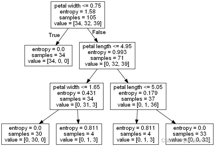

GraphViz可以在www.graphviz.org免费下载.