100 deep learning cases | day 41 - convolutional neural network (CNN): urbansound 8K audio classification (speech recognition)

• Running environment ：python3
• author ：K Students
• From column ：《 Deep learning 100 example 》
• Select columns ：《 Novice introduction and deep learning 》
• Recommendation column ：《Matplotlib course 》
• 🧿 Excellent column ：《Python introduction 100 topic 》

---

My environment ：

• Language environment ：Python3.6.5
• compiler ：jupyter notebook
• Deep learning environment ：TensorFlow2.4.1
• The graphics card （GPU）：NVIDIA GeForce RTX 3080
• Data address ：【 Portal 】

Our code flow chart is as follows ：

One 、 preparation

Hello everyone , I am a K Students ！

Today, I would like to share with you a practical case of audio classification .

The data set used is UrbanSound8K, The dataset contains data from 10 There are three categories of urban sound 8732 A tag sound excerpt (<=4s)：air_conditioner、car_horn、children_playing、dog_bark、drilling、enginge_idling、gun_shot、jackhammer、siren and street_music, Data exist separately fold1-fold10 Wait in ten folders .

In addition to sound excerpts , One is also provided CSV file , It contains metadata about each excerpt .

Methods to introduce

1. Yes 3 A basic method of extracting features from audio files ：

   a) Using audio files mffcs data
   b) Use the spectrum image of audio , Then convert it into data points （ Just like you did with the image ）. This can be used Librosa Of mel_spectogram function Easy to finish
   c) Combine these two features to build a better model . （ It takes a lot of time to read and extract data ）.

2. I choose to use the second method .

3. Labels have been converted to classification data for classification .

4. CNN Has been used as the main layer for classifying data

1. Import the required Library

# Basic Libraries

import pandas as pd
import numpy as np

pd.plotting.register_matplotlib_converters()
import matplotlib.pyplot as plt
%matplotlib inline
import seaborn as sns

from sklearn.model_selection import train_test_split
from sklearn.metrics import classification_report
from sklearn.model_selection import GridSearchCV
from sklearn.preprocessing import MinMaxScaler
from tensorflow.keras.models import Sequential
from tensorflow.keras.layers import Conv2D, Flatten, Dense, MaxPool2D, Dropout
from tensorflow.keras.utils import to_categorical 
import os,glob,skimage,librosa
import librosa.display

import warnings
warnings.filterwarnings("ignore")             # Ignore the warning 

2. Analyze data type and format

analysis CSV data

df = pd.read_csv("./41-data/UrbanSound8K.csv")

df.head()

	slice_file_name	fsID	start	end	salience	fold	classID	class
0	100032-3-0-0.wav	100032	0.0	0.317551	1	5	3	dog_bark
1	100263-2-0-117.wav	100263	58.5	62.500000	1	5	2	children_playing
2	100263-2-0-121.wav	100263	60.5	64.500000	1	5	2	children_playing
3	100263-2-0-126.wav	100263	63.0	67.000000	1	5	2	children_playing
4	100263-2-0-137.wav	100263	68.5	72.500000	1	5	2	children_playing

Name

• slice_file_name： Audio file name . The naming format is : [fsID]-[classID]-[occurrenceID]-[sliceID].wav

  • [fsID]： Extract extracts from （ fragment ） Recorded Freesound ID
  • [classID]： Category ID
  • [occurrenceID]： A numeric identifier , Sounds used to distinguish different events in the original recording
  • [sliceID]： A numeric identifier , Used to distinguish different slices obtained from the same event

• fsID： Extract extracts from （ fragment ） Recorded Freesound ID

• start： original Freesound The start time of the clip in the recording

• end： original Freesound The end time of the slice in the recording

• salience： The voice （ subjective ） Significance level . 1 = prospects ,2 = background .

• fold： altogether 1-10,10 A folder

• classID： Digital identifier of the sound category ：

  • 0 = air_conditioner
  • 1 = car_horn
  • 2 = children_playing
  • 3 = dog_bark
  • 4 = drilling
  • 5 = engine_idling
  • 6 = gun_shot
  • 7 = jackhammer
  • 8 = siren
  • 9 = street_music

Use Librosa Analyze random sound samples

a,b = librosa.load() Return value ：

• a: Audio signal value , The type is ndarray
• b: Sampling rate

3. Data presentation

import IPython.display as ipd
ipd.Audio('./41-data/fold5/100263-2-0-117.wav')

dataSample, sampling_rate = librosa.load('./41-data/fold5/100032-3-0-0.wav')

plt.figure(figsize=(10, 3))

D = librosa.amplitude_to_db(np.abs(librosa.stft(dataSample)), ref=np.max)
librosa.display.specshow(D, y_axis='linear')

plt.colorbar(format='%+2.0f dB')
plt.title('Linear-frequency power spectrogram')
plt.show()

arr  = np.array(df["slice_file_name"])
fold = np.array(df["fold"])
cla  = np.array(df["class"])

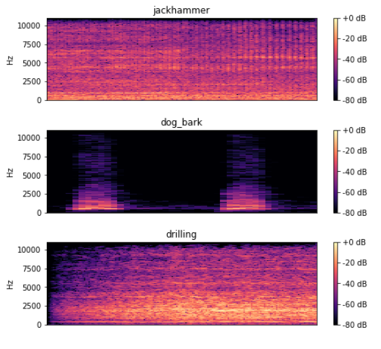
for i in range(192, 197, 2):
    plt.figure(figsize=(8, 2))
    
    path = './41-data/fold' + str(fold[i]) + '/' + arr[i]
    data, sampling_rate = librosa.load(path)
    
    D = librosa.amplitude_to_db(np.abs(librosa.stft(data)), ref=np.max)
    librosa.display.specshow(D, y_axis='linear')
    plt.colorbar(format='%+2.0f dB')
    plt.title(cla[i])

Two 、 Feature extraction and data set construction

Let's see how to use it librosa.feature.melspectrogram() The data extracted by the function shape

arr = librosa.feature.melspectrogram(y=data, sr=sampling_rate)
arr.shape

(128, 173)

1. Data feature extraction

feature = []
label   = []

def parser():
    #  Load the file and extract the features 
    for i in range(8732):
        if i%1000 == 0:
            print(" Has been extracted %d Data characteristics "%i)
            
        file_name = './41-data/fold' + str(df["fold"][i]) + '/' + df["slice_file_name"][i]
        X, sample_rate = librosa.load(file_name, res_type='kaiser_fast') 
        #  Extract the spectrum to form an image array 
        mels = np.mean(librosa.feature.melspectrogram(y=X, sr=sample_rate).T,axis=0)        
        feature.append(mels)
        label.append(df["classID"][i])
    print(" Data feature extraction is complete ！")
    return [feature, label]

temp = parser()

 Has been extracted 0 Data characteristics 
 Has been extracted 1000 Data characteristics 
 Has been extracted 2000 Data characteristics 
 Has been extracted 3000 Data characteristics 
 Has been extracted 4000 Data characteristics 
 Has been extracted 5000 Data characteristics 
 Has been extracted 6000 Data characteristics 
 Has been extracted 7000 Data characteristics 
 Has been extracted 8000 Data characteristics 
 Data feature extraction is complete ！

temp_numpy = np.array(temp).transpose()

X_ = temp_numpy[:, 0]
Y_ = temp_numpy[:, 1]

X = np.array([X_[i] for i in range(8732)])
Y = to_categorical(Y_)

print(X.shape, Y.shape)

(8732, 128) (8732, 10)

2. Dataset construction

X_train, X_test, Y_train, Y_test = train_test_split(X, Y, random_state = 1)

X_train = X_train.reshape(6549, 16, 8, 1)
X_test  = X_test.reshape(2183, 16, 8, 1)

input_dim = (16, 8, 1)

3、 ... and 、 Build models and train

model = Sequential()

model.add(Conv2D(64, (3, 3), padding = "same", activation = "tanh", input_shape = input_dim))
model.add(MaxPool2D(pool_size=(2, 2)))
model.add(Conv2D(128, (3, 3), padding = "same", activation = "tanh"))
model.add(MaxPool2D(pool_size=(2, 2)))
model.add(Dropout(0.1))
model.add(Flatten())
model.add(Dense(1024, activation = "tanh"))
model.add(Dense(10, activation = "softmax"))

model.compile(optimizer = 'adam', loss = 'categorical_crossentropy', metrics = ['accuracy'])

model.fit(X_train, Y_train, epochs = 90, batch_size = 50, validation_data = (X_test, Y_test))

Epoch 1/90
131/131 [==============================] - 3s 4ms/step - loss: 1.5368 - accuracy: 0.4717 - val_loss: 1.3617 - val_accuracy: 0.5144
Epoch 2/90
131/131 [==============================] - 0s 2ms/step - loss: 1.1502 - accuracy: 0.6091 - val_loss: 1.1119 - val_accuracy: 0.6326
  ......
131/131 [==============================] - 0s 2ms/step - loss: 0.0481 - accuracy: 0.9835 - val_loss: 0.8535 - val_accuracy: 0.8653
Epoch 89/90
131/131 [==============================] - 0s 2ms/step - loss: 0.0511 - accuracy: 0.9818 - val_loss: 0.7716 - val_accuracy: 0.8694
Epoch 90/90
131/131 [==============================] - 0s 2ms/step - loss: 0.0502 - accuracy: 0.9829 - val_loss: 0.8673 - val_accuracy: 0.8630

model.summary()

Model: "sequential"
_________________________________________________________________
Layer (type)                 Output Shape              Param #   
=================================================================
conv2d (Conv2D)              (None, 16, 8, 64)         640       
_________________________________________________________________
max_pooling2d (MaxPooling2D) (None, 8, 4, 64)          0         
_________________________________________________________________
conv2d_1 (Conv2D)            (None, 8, 4, 128)         73856     
_________________________________________________________________
max_pooling2d_1 (MaxPooling2 (None, 4, 2, 128)         0         
_________________________________________________________________
dropout (Dropout)            (None, 4, 2, 128)         0         
_________________________________________________________________
flatten (Flatten)            (None, 1024)              0         
_________________________________________________________________
dense (Dense)                (None, 1024)              1049600   
_________________________________________________________________
dense_1 (Dense)              (None, 10)                10250     
=================================================================
Total params: 1,134,346
Trainable params: 1,134,346
Non-trainable params: 0
_________________________________________________________________

predictions = model.predict(X_test)
score = model.evaluate(X_test, Y_test)
print(score)

69/69 [==============================] - 0s 1ms/step - loss: 0.8673 - accuracy: 0.8630
[0.8672816753387451, 0.8630325198173523]