当前位置:网站首页>Machine learning theory (7): kernel function kernels -- a way to help SVM realize nonlinear decision boundary
Machine learning theory (7): kernel function kernels -- a way to help SVM realize nonlinear decision boundary
2022-04-23 18:33:00 【Flying warm】
List of articles
About SVM The principle and why SVM Always choose the big one margin Decide the boundary , I'm in the article :
https://blog.csdn.net/qq_42902997/article/details/124310782
It is expounded in , If you don't understand, you can review
review SVM The goal of optimization
C Σ i = 1 m y i c o s t 1 ( θ T x i ) + ( 1 − y i ) c o s t 0 ( θ T x i ) + 1 2 Σ j = 1 n θ j 2 ( 1 ) C\Sigma_{i=1}^m{y_i}cost_1(\theta^Tx_i)+(1-y_i)cost_0(\theta^Tx_i)+\frac{1}{2}\Sigma_{j=1}^n\theta_j^2~~~~~~~~~~(1) CΣi=1myicost1(θTxi)+(1−yi)cost0(θTxi)+21Σj=1nθj2 (1)
- We all know SVM Is a linear classifier , Then face the following linear inseparable scene :

- If you want to implement classification , Then it is absolutely impossible to use a linear classifier to realize , Therefore, we want to introduce polynomials to construct higher-order features to achieve the purpose of the final nonlinear classification .
- Look at the formula given in the figure ; For all the characteristics of a sample x ⃗ = { x 1 , x 2 } \vec{x}=\{x_1,x_2\} x={
x1,x2}; Try to make higher-order features based on these features x 1 x 2 , x 1 2 , x 2 2 x_1x_2, x_1^2, x_2^2 x1x2,x12,x22 And so on to construct a nonlinear decision boundary :

- Well, along this line , We use a more general form to express , Because our goal is to make higher-order features , So we use θ 0 + θ 1 f 1 + θ 2 f 2 + . . . + θ n f n \theta_0 + \theta_1f_1 + \theta_2f_2+...+\theta_nf_n θ0+θ1f1+θ2f2+...+θnfn To represent our decision boundary ; among n n n Is the number of features we end up using ; And these f 1 , f 2 , . . . , f n f_1, f_2, ..., f_n f1,f2,...,fn It's the new feature we're going to use .
- In the example above , f 1 = x 1 , f 2 = x 2 , f 3 = x 1 x 2 , f 4 = x 1 2 , f 5 = x 2 2 , . . . f_1=x_1, f_2=x_2, f_3=x_1x_2, f_4=x_1^2,f_5=x_2^2, ... f1=x1,f2=x2,f3=x1x2,f4=x12,f5=x22,...
- Now comes the question , How to ensure that we f 1 , . . . , f n f_1,...,f_n f1,...,fn Is it effective ?
How to construct f 1 , . . . , f n f_1,...,f_n f1,...,fn
landmark & similarity
- Use to measure the current sample points and some landmark( Marker points ) Similarity is used to generate f 1 , . . . , f n f_1,...,f_n f1,...,fn.
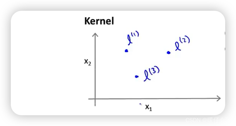
Still use the example mentioned above , For each sample point x x x Use two features to represent x ⃗ = { x 1 , x 2 } \vec{x}=\{x_1,x_2\} x={ x1,x2}, At this time, we assume that 3 3 3 Different landmarks( This will be explained in detail later landmarks How it was chosen )
Next , We measure the samples separately x x x And these three landmarks Similarity as f 1 , . . . , f n f_1,...,f_n f1,...,fn The process of defining :
- f 1 = s i m i l a r i t y ( x , l ( 1 ) ) f_1=similarity(x,l^{(1)}) f1=similarity(x,l(1))
- f 2 = s i m i l a r i t y ( x , l ( 2 ) ) f_2=similarity(x,l^{(2)}) f2=similarity(x,l(2))
- f 3 = s i m i l a r i t y ( x , l ( 3 ) ) f_3=similarity(x,l^{(3)}) f3=similarity(x,l(3))
And this s i m i l a r i t y similarity similarity We use Gaussian kernel function to define ( I'll explain it in detail later )
That is, we use a :
s i m i l a r i t y ( x , z ) = e x p ( − ∣ ∣ x − z ∣ ∣ 2 2 σ 2 ) similarity(x,z)=exp(-\frac{||x-z||^2}{2\sigma^2}) similarity(x,z)=exp(−2σ2∣∣x−z∣∣2)
therefore , above f 1 , . . f 3 f_1,..f_3 f1,..f3 Can be transformed into :- f 1 = e x p ( − ∣ ∣ x − l ( 1 ) ∣ ∣ 2 2 σ 2 ) f_1=exp(-\frac{||x-l^{(1)}||^2}{2\sigma^2}) f1=exp(−2σ2∣∣x−l(1)∣∣2)
- f 2 = e x p ( − ∣ ∣ x − l ( 2 ) ∣ ∣ 2 2 σ 2 ) f_2=exp(-\frac{||x-l^{(2)}||^2}{2\sigma^2}) f2=exp(−2σ2∣∣x−l(2)∣∣2)
- f 3 = e x p ( − ∣ ∣ x − l ( 3 ) ∣ ∣ 2 2 σ 2 ) f_3=exp(-\frac{||x-l^{(3)}||^2}{2\sigma^2}) f3=exp(−2σ2∣∣x−l(3)∣∣2)
Note: ∣ ∣ x − l ( 1 ) ∣ ∣ 2 = Σ i = 1 m ( x i − l i ) 2 ||x-l^{(1)}||^2=\Sigma_{i=1}^m(x_i-l_i)^2 ∣∣x−l(1)∣∣2=Σi=1m(xi−li)2 m m m It's a sample x x x Number of features used in , Here it is. x 1 , x 2 x_1,x_2 x1,x2 Two characteristics, so m = 2 m=2 m=2
You can see , Under the definition of this function , If x x x and l ( i ) l^{(i)} l(i) Are very similar , Then the result of the kernel function will be close to f i ≈ e x p ( − 0 2 σ 2 ) ≈ 1 f_i\approx exp(-\frac{0}{2\sigma^2})\approx1 fi≈exp(−2σ20)≈1 ; contrary , If x x x and l ( i ) l^{(i)} l(i) Far away , Then the result is close to 0 0 0.
So we can think of f 1 , . . . , f n f_1,...,f_n f1,...,fn Measured x x x This sample to these landmark Similar procedures ( Distance metric ); And these f 1 , . . . , f n f_1,...,f_n f1,...,fn Become a component x x x This sample is n n n Features
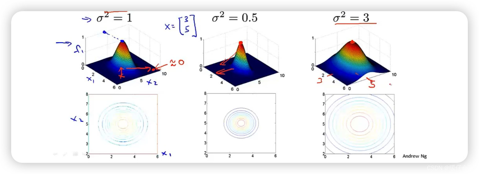
For ease of understanding , We visualize Gaussian kernel function
As you can see from the picture , When l ( 1 ) l^{(1)} l(1) The closer you are to x x x, Then the result of passing through the Gaussian kernel function is closer to the center of the graph , The closer the value is 1 1 1; contrary , If it is farther away, the value is closer to 0 0 0
We can also draw a simple conclusion : Standard deviation of Gaussian kernel function σ \sigma σ The size of determines the smoothness of the distribution , For example, choose different σ \sigma σ The distribution is different :

How to generate nonlinear boundary
- Let's say we've got through calculation θ 0 , θ 1 , . . . θ 3 \theta_0, \theta_1,...\theta_3 θ0,θ1,...θ3, Their values are shown in the figure :

- If there is a sample at this time x x x In the position in the figure : distance l ( 1 ) l^{(1)} l(1) Very close , But distance l ( 2 ) , l ( 3 ) l^{(2)},l^{(3)} l(2),l(3) Far away , Then we can think that f 1 ≈ 1 ; f 2 , f 3 ≈ 0 f_1\approx1; f_2, f_3\approx0 f1≈1;f2,f3≈0 Calculate by bringing in the formula , The final prediction we can get is > = 0 >=0 >=0 Of , Positive sample .

- If there is another sample at this time x x x, Three l ( i ) l^{(i)} l(i) Far away : According to the same steps, we can calculate that his prediction label is < 0 <0 <0 Of , Negative samples .
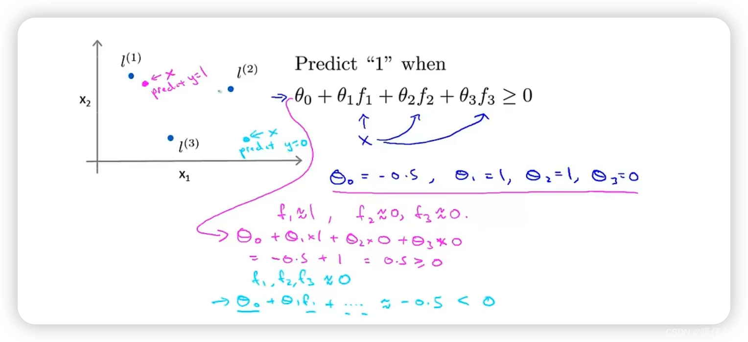
- If the sample size is large enough , You'll find that : The final prediction result of these samples actually depends on all landmarks, The resulting decision boundary will become a nonlinear decision boundary . All samples inside the red boundary will be judged as positive samples , All samples outside the red boundary will be judged as negative samples .

How to choose landmarks
-
In fact, you may have thought of , We can use all the sample points in this dataset X = x ( 1 ) , x ( 2 ) , . . . , x ( n ) X={x^{(1)},x^{(2)},...,x^{(n)}} X=x(1),x(2),...,x(n) As these landmarks l ( 1 ) = x ( 1 ) , l ( 2 ) = x ( 2 ) , . . . , l ( n ) = x ( n ) l^{(1)}=x^{(1)},l^{(2)}=x^{(2)},...,l^{(n)}=x^{(n)} l(1)=x(1),l(2)=x(2),...,l(n)=x(n)
-
The similarity of samples can be rewritten into the following formula :
- f 1 = e x p ( − ∣ ∣ x − x ( 1 ) ∣ ∣ 2 2 σ 2 ) f_1=exp(-\frac{||x-x^{(1)}||^2}{2\sigma^2}) f1=exp(−2σ2∣∣x−x(1)∣∣2)
- f 2 = e x p ( − ∣ ∣ x − x ( 2 ) ∣ ∣ 2 2 σ 2 ) f_2=exp(-\frac{||x-x^{(2)}||^2}{2\sigma^2}) f2=exp(−2σ2∣∣x−x(2)∣∣2)
- f 3 = e x p ( − ∣ ∣ x − x ( 3 ) ∣ ∣ 2 2 σ 2 ) f_3=exp(-\frac{||x-x^{(3)}||^2}{2\sigma^2}) f3=exp(−2σ2∣∣x−x(3)∣∣2)
.
.
. - f n = e x p ( − ∣ ∣ x − x ( n ) ∣ ∣ 2 2 σ 2 ) f_n=exp(-\frac{||x-x^{(n)}||^2}{2\sigma^2}) fn=exp(−2σ2∣∣x−x(n)∣∣2)
-
thus , Every sample x ( i ) x^{(i)} x(i) Eigenvector of x ( i ) ⃗ \vec{x^{(i)}} x(i) By the original { x 1 ( i ) , x 2 ( i ) } \{x^{(i)}_1,x^{(i)}_2\} { x1(i),x2(i)} Turned into f ( i ) ⃗ = { f 1 ( i ) , f 2 ( i ) , . . . , f n ( i ) } \vec{f^{(i)}}=\{f^{(i)}_1, f^{(i)}_2,..., f^{(i)}_n\} f(i)={ f1(i),f2(i),...,fn(i)}; In fact, we omit the intercept feature here f 0 ( i ) f^{(i)}_0 f0(i), If you want to add it, it's also very simple , f ( i ) ⃗ = { f 0 ( i ) , f 1 ( i ) , f 2 ( i ) , . . . , f n ( i ) } \vec{f^{(i)}}=\{f^{(i)}_0, f^{(i)}_1, f^{(i)}_2,..., f^{(i)}_n\} f(i)={ f0(i),f1(i),f2(i),...,fn(i)}
-
The same is about to change , It's with this n n n Dimension vector ( If you count f 0 f_0 f0 Namely n + 1 n+1 n+1 dimension ) The vector corresponds to θ ⃗ = θ 0 , . . . , θ n \vec{\theta}={\theta_0,..., \theta_n} θ=θ0,...,θn
-
We finally passed θ T ⋅ f ⃗ = θ 0 f 0 + . . . + θ n f n > = 0 \theta^T \cdot \vec{f} = \theta_0f_0+...+\theta_nf_n>=0 θT⋅f=θ0f0+...+θnfn>=0 To predict a positive sample .
SVM Combined kernel function
-
Combine the above , Let's look back SVM The objective function of , For a containing m m m The data set of 2 samples :
C Σ i = 1 m y i c o s t 1 ( θ T x ( i ) ) + ( 1 − y i ) c o s t 0 ( θ T x ( i ) ) + 1 2 Σ j = 1 n θ j 2 ( 1 ) C\Sigma_{i=1}^m{y_i}cost_1(\theta^Tx^{(i)})+(1-y_i)cost_0(\theta^Tx^{(i)})+\frac{1}{2}\Sigma_{j=1}^n\theta_j^2~~~~~~~~~~(1) CΣi=1myicost1(θTx(i))+(1−yi)cost0(θTx(i))+21Σj=1nθj2 (1) -
We can rewrite this optimization goal as :
C Σ i = 1 m y i c o s t 1 ( θ T ⋅ f ( i ) ⃗ ) + ( 1 − y i ) c o s t 0 ( θ T ⋅ f ( i ) ⃗ ) + 1 2 Σ j = 1 n θ j 2 ( 2 ) C\Sigma_{i=1}^m{y_i}cost_1(\theta^T\cdot \vec{f^{(i)}})+(1-y_i)cost_0(\theta^T\cdot \vec{f^{(i)}})+\frac{1}{2}\Sigma_{j=1}^n\theta_j^2~~~~~~~~~~(2) CΣi=1myicost1(θT⋅f(i))+(1−yi)cost0(θT⋅f(i))+21Σj=1nθj2 (2) -
That is to put the original x x x The feature vector is transformed into a new one based on f f f Eigenvector of ; Now the number of samples is m m m.
-
At the same time , Regularized part of n n n It originally represented a sample x ( i ) x^{(i)} x(i) The number of effective features in , Now this quantity can also be replaced by m m m 了 , Because the number of effective features is the number of samples , So the formula is optimized again to :
C Σ i = 1 m y i c o s t 1 ( θ T ⋅ f ( i ) ⃗ ) + ( 1 − y i ) c o s t 0 ( θ T ⋅ f ( i ) ⃗ ) + 1 2 Σ j = 1 m θ j 2 ( 2 ) C\Sigma_{i=1}^m{y_i}cost_1(\theta^T\cdot \vec{f^{(i)}})+(1-y_i)cost_0(\theta^T\cdot \vec{f^{(i)}})+\frac{1}{2}\Sigma_{j=1}^m\theta_j^2~~~~~~~~~~(2) CΣi=1myicost1(θT⋅f(i))+(1−yi)cost0(θT⋅f(i))+21Σj=1mθj2 (2)
- there j = 1... m j=1...m j=1...m The feature that cannot contain intercept , That is, this part of regularization , There can only be at most m m m The item , Because the intercept feature is not included in the optimization of regularization, it cannot be written as j = 0... m j=0...m j=0...m.
- So the regular term can also be written as θ T ⋅ θ ( i g n o r i n g θ 0 ) \theta^T\cdot \theta ~~~(ignoring~~ \theta_0) θT⋅θ (ignoring θ0)
版权声明
本文为[Flying warm]所创,转载请带上原文链接,感谢
https://yzsam.com/2022/04/202204231826143997.html
边栏推荐
- 使用 bitnami/postgresql-repmgr 镜像快速设置 PostgreSQL HA
- 昇腾 AI 开发者创享日全国巡回首站在西安成功举行
- Analysez l'objet promise avec le noyau dur (Connaissez - vous les sept API communes obligatoires et les sept questions clés?)
- Rust: the output information of println is displayed during the unit test
- 串口调试工具cutecom和minicom
- Robocode tutorial 8 - advanced robot
- CISSP certified daily knowledge points (April 18, 2022)
- CISSP certified daily knowledge points (April 15, 2022)
- 【数学建模】—— 层次分析法(AHP)
- Daily CISSP certification common mistakes (April 12, 2022)
猜你喜欢

Install the yapiupload plug-in in idea and upload the API interface to the Yapi document
机器学习理论之(7):核函数 Kernels —— 一种帮助 SVM 实现非线性化决策边界的方式
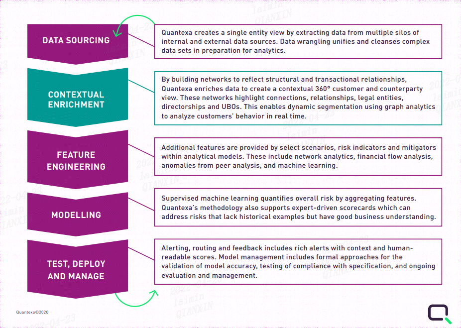
Quantexa CDI(场景决策智能)Syneo平台介绍

昇腾 AI 开发者创享日全国巡回首站在西安成功举行
Win1远程出现“这可能是由于credssp加密oracle修正”解决办法

Differences between SSD hard disk SATA interface and m.2 interface (detailed summary)

Ctfshow - web362 (ssti)
WIN1 remote "this may be due to credssp encryption Oracle correction" solution
QT reading and writing XML files (including source code + comments)

Teach you to quickly rename folder names in a few simple steps
随机推荐
CISSP certified daily knowledge points (April 19, 2022)
Keil RVMDK compiled data type
According to the result set queried by SQL statement, it is encapsulated as JSON
QT error: no matching member function for call to ‘connect‘
Daily network security certification test questions (April 15, 2022)
JD-FreeFuck 京东薅羊毛控制面板 后台命令执行漏洞
登录和发布文章功能测试
多功能工具箱微信小程序源码
Dynamically add default fusing rules to feign client based on sentinel + Nacos
Cutting permission of logrotate file
使用 bitnami/postgresql-repmgr 镜像快速设置 PostgreSQL HA
Daily CISSP certification common mistakes (April 12, 2022)
回路-通路
Solution to Chinese garbled code after reg file is imported into the registry
数据库上机实验四(数据完整性与存储过程)
【ACM】455. 分发饼干(1. 大饼干优先喂给大胃口;2. 遍历两个数组可以只用一个for循环(用下标索引--来遍历另一个数组))
ctfshow-web362(SSTI)
根据快递单号查询物流查询更新量
Rust: shared variable in thread pool
If condition judgment in shell language